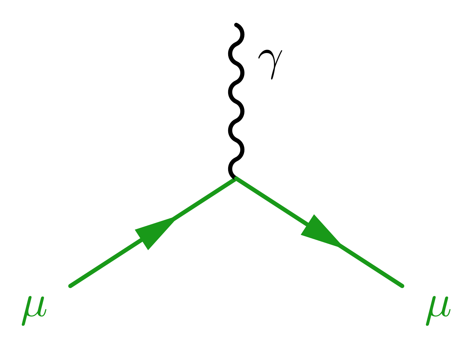
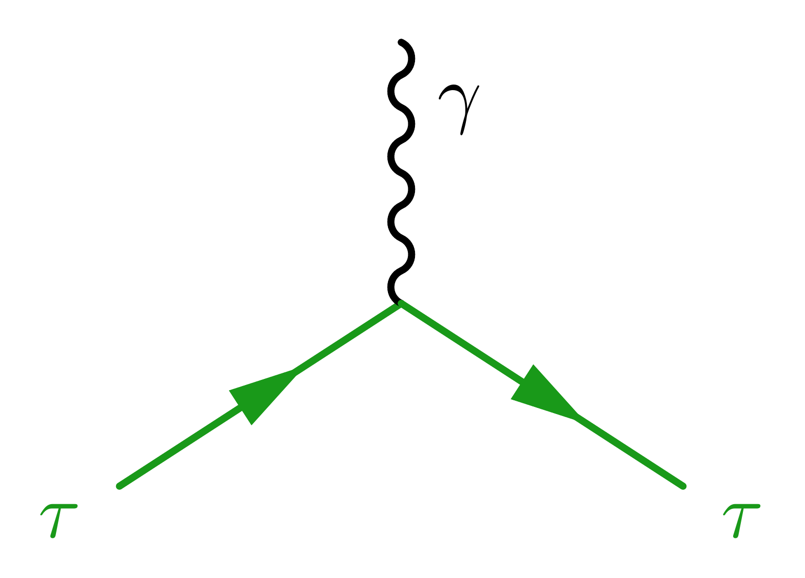
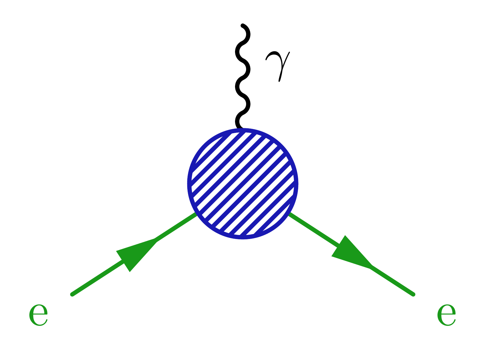
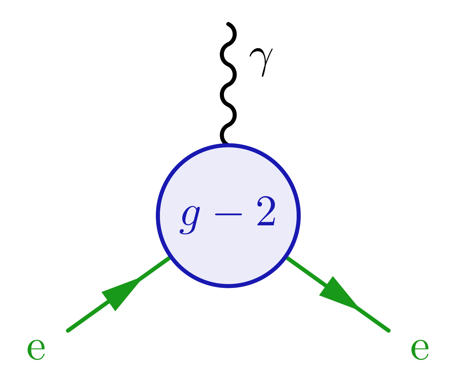
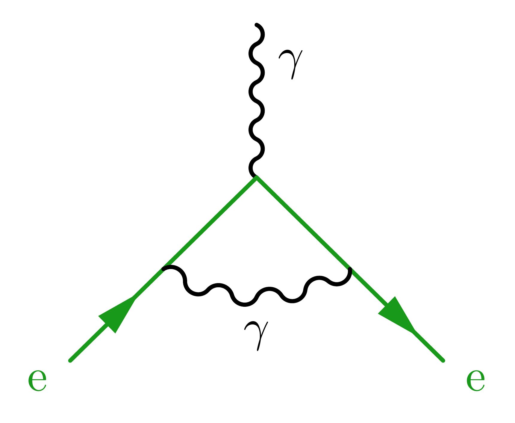
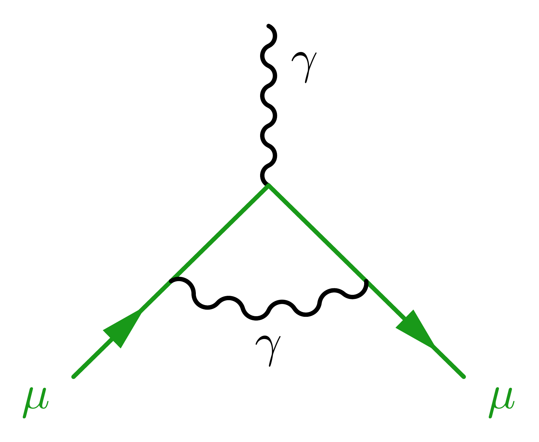
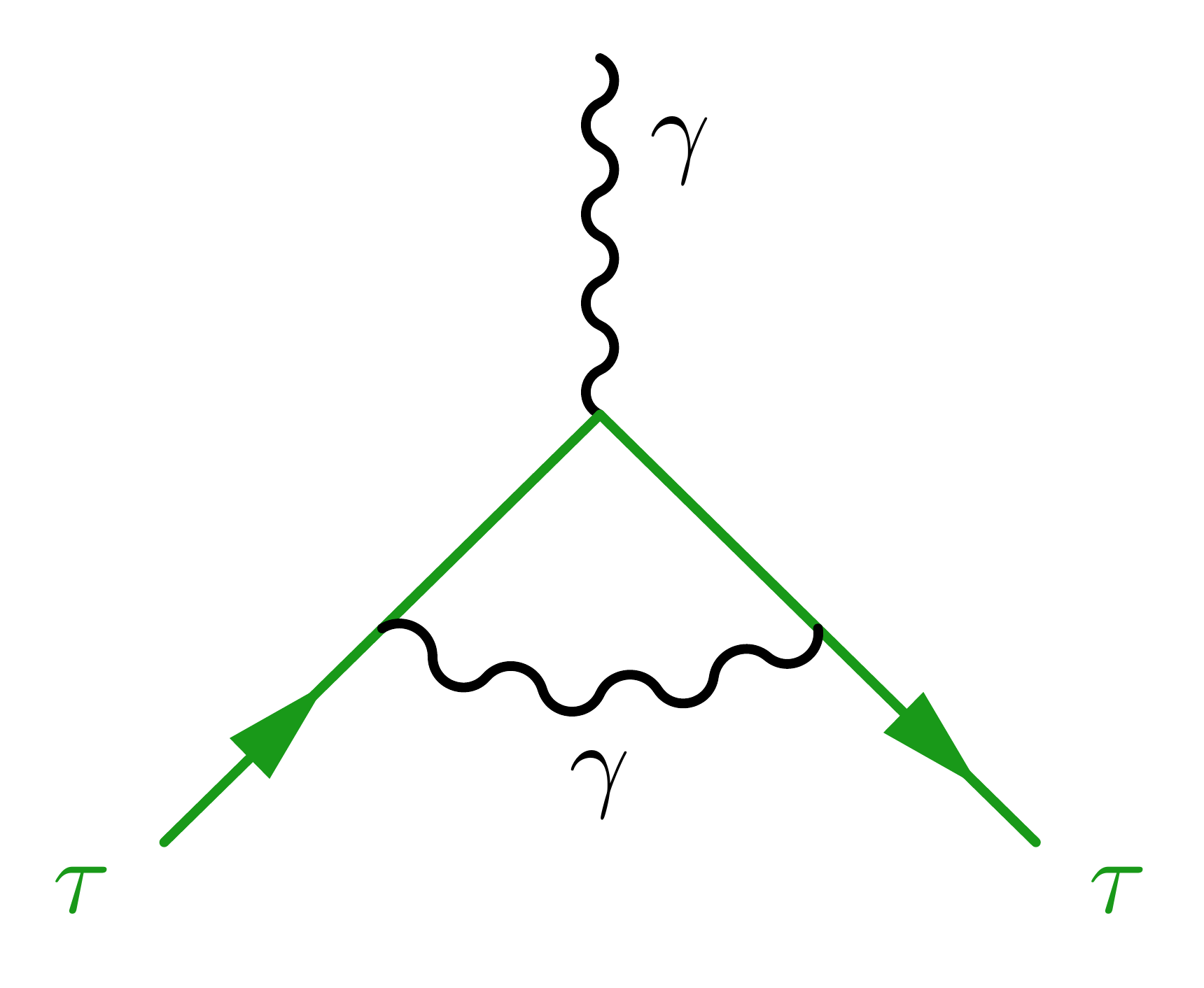
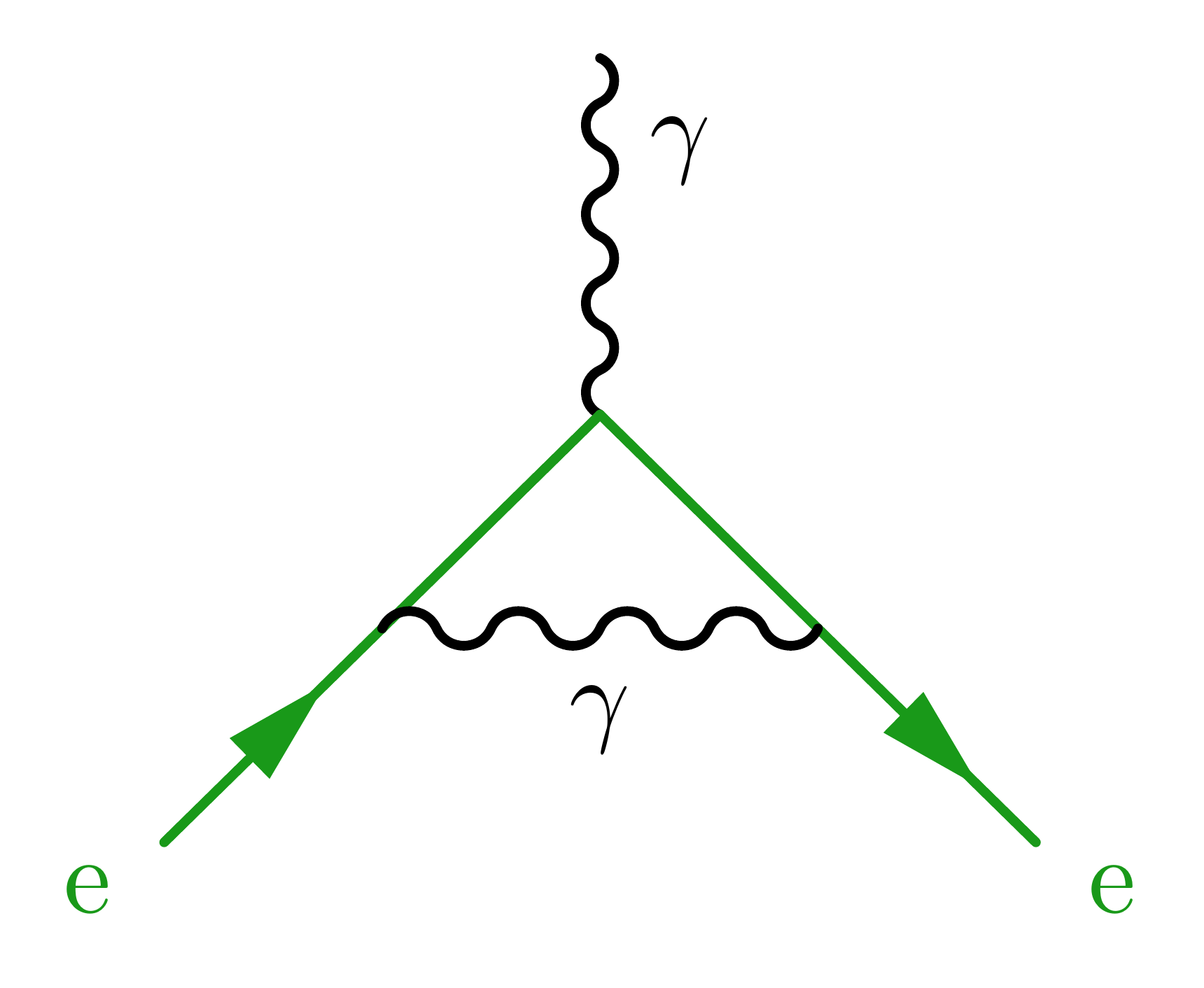
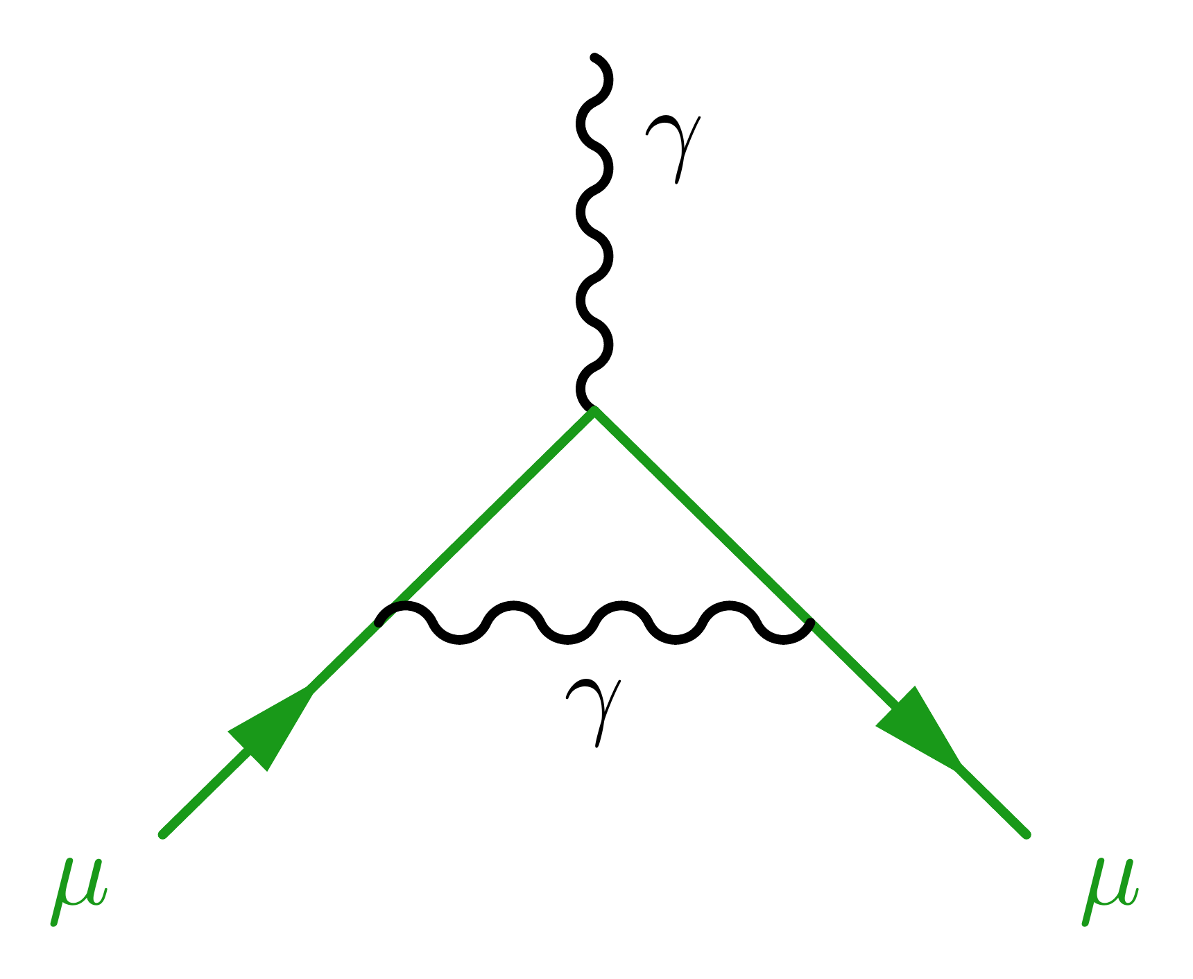
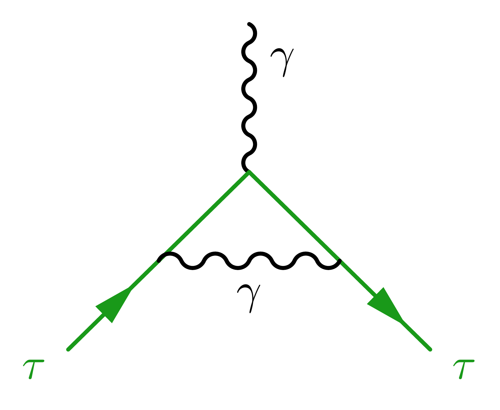
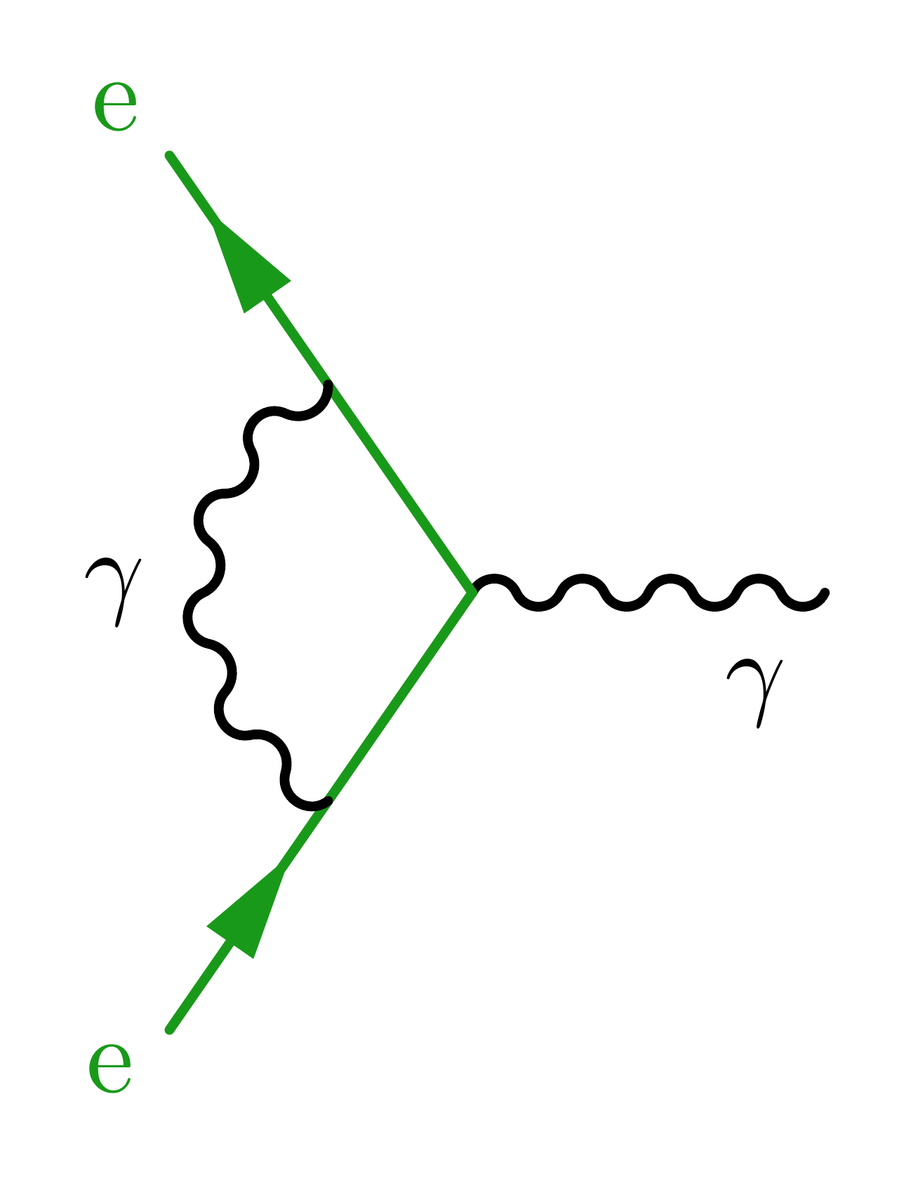
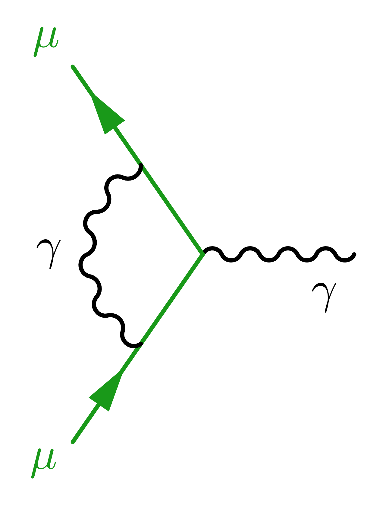
Below are some code examples the leading contribution to the anomalous magnetic moment (g-2), which is the one-loop diagram that was famously calculated by Julian Schwinger in 1948. Some of the diagrams below were presented in this seminar talk (UZH, 2024).
Click on a diagram to jump to the code & download links below: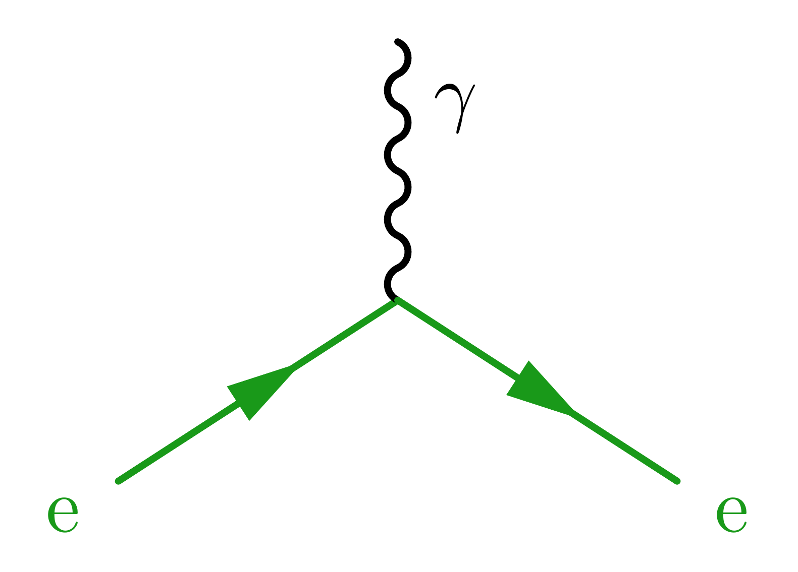

\documentclass[11pt,border=4pt]{standalone}
\usepackage{feynmp-auto}
\usepackage{xcolor}
\definecolor{collep}{rgb}{.1,.6,.1} % lepton (green)
\begin{document}
\begin{fmffile}{feyngraph}
  \fmfframe(2,2)(6,2){ % padding (L,T)(R,B)
  \begin{fmfgraph*}(80,70) % canvas (W,H)
    % line style
    \fmfset{wiggly_len}{12} % boson wavelength
    \fmfset{wiggly_slope}{65} % boson slope of waves
    % external vertices
    \fmfbottom{f2,f1}
    \fmftop{g}
    % main process
    \fmf{boson,t=1.4}{g,v} % photon
    \fmf{fermion,f=(.1,,.6,,.1)}{f2,v,f1} % lepton pair
    % labels
    \fmfv{l.a=-50,l.d=8,l=$\gamma$}{g}
    \fmfv{l.a=-25,l=\color{collep}e}{f1}
    \fmfv{l.a=-155,l=\color{collep}e}{f2}
  \end{fmfgraph*}
  } % close \fmfframe
\end{fmffile}
\end{document}
\documentclass[11pt,border=4pt]{standalone}
\usepackage{feynmp-auto}
\usepackage{xcolor}
\definecolor{collep}{rgb}{.1,.6,.1} % lepton (green)
\begin{document}
\begin{fmffile}{feyngraph}
\fmfframe(2,2)(6,2){ % padding (L,T)(R,B)
\begin{fmfgraph*}(80,70) % canvas (W,H)
% line style
\fmfset{wiggly_len}{12} % boson wavelength
\fmfset{wiggly_slope}{65} % boson slope of waves
% external vertices
\fmfbottom{f2,f1}
\fmftop{g}
% main process
\fmf{boson,t=1.4}{g,v} % photon
\fmf{fermion,f=(.1,,.6,,.1)}{f2,v,f1} % lepton pair
% labels
\fmfv{l.a=-50,l.d=8,l=$\gamma$}{g}
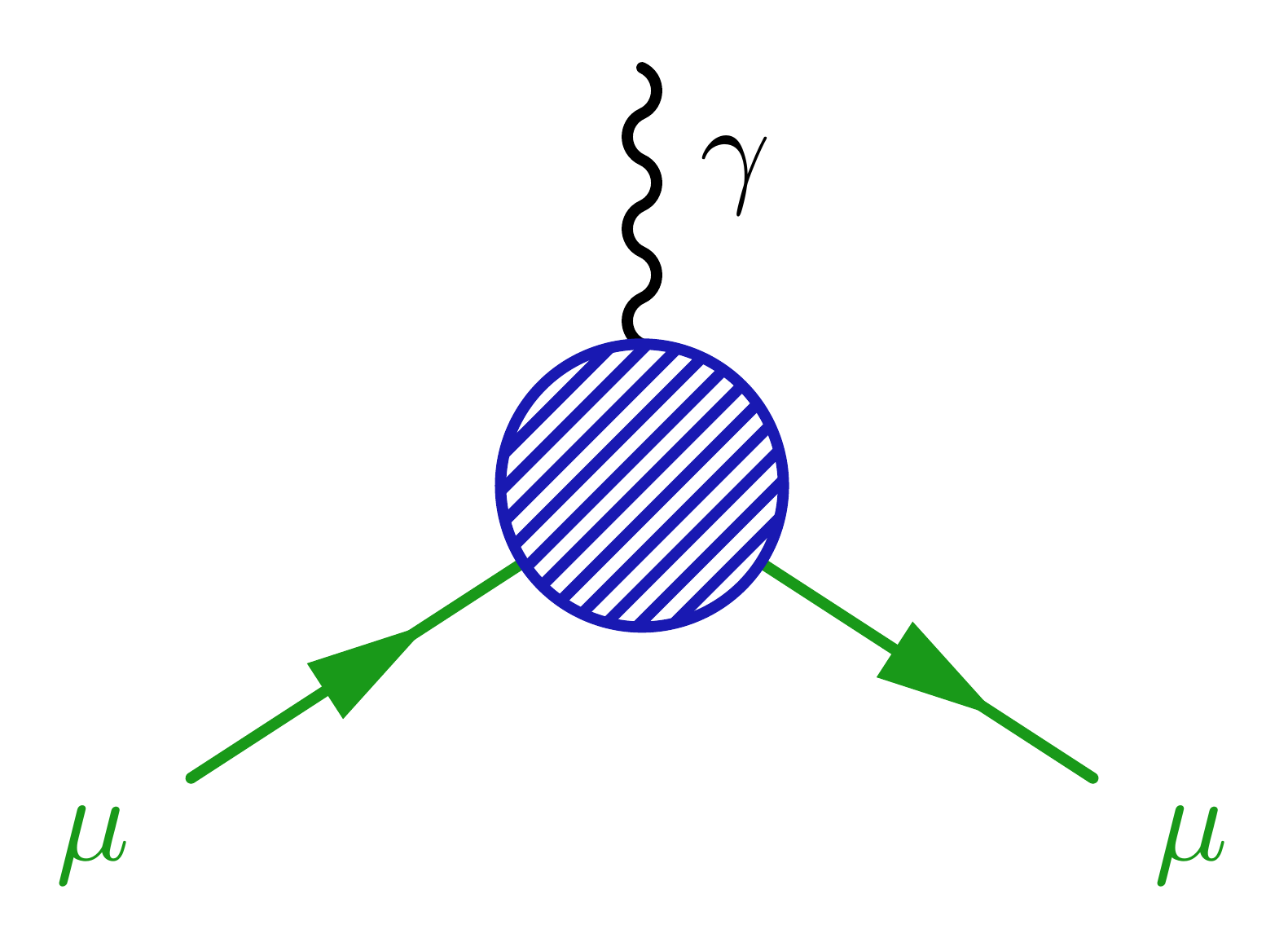
\fmfv{l.a=-25,l=\color{collep}$\mu$}{f1}
\fmfv{l.a=-155,l=\color{collep}$\mu$}{f2}
\end{fmfgraph*}
} % close \fmfframe
\end{fmffile}
\end{document}
\documentclass[11pt,border=4pt]{standalone}
\usepackage{feynmp-auto}
\usepackage{xcolor}
\definecolor{collep}{rgb}{.1,.6,.1} % lepton (green)
\begin{document}
\begin{fmffile}{feyngraph}
  \fmfframe(2,2)(6,2){ % padding (L,T)(R,B)
  \begin{fmfgraph*}(80,70) % canvas (W,H)
    % line style
    \fmfset{wiggly_len}{12} % boson wavelength
    \fmfset{wiggly_slope}{65} % boson slope of waves
    % external vertices
    \fmfbottom{f2,f1}
    \fmftop{g}
    % main process
    \fmf{boson,t=1.4}{g,v} % photon
    \fmf{fermion,f=(.1,,.6,,.1)}{f2,v,f1} % lepton pair
    % labels
    \fmfv{l.a=-50,l.d=8,l=$\gamma$}{g}
    \fmfv{l.a=-25,l=\color{collep}$\tau$}{f1}
    \fmfv{l.a=-155,l=\color{collep}$\tau$}{f2}
  \end{fmfgraph*}
  } % close \fmfframe
\end{fmffile}
\end{document}
\documentclass[11pt,border=4pt]{standalone}
\usepackage{feynmp-auto}
\usepackage{xcolor}
\definecolor{collep}{rgb}{.1,.6,.1} % lepton (green)
\definecolor{colvtx}{rgb}{.1,.1,.7} % vertex (dark blue)
\begin{document}
\begin{fmffile}{feyngraph}
  \fmfframe(2,2)(6,2){ % padding (L,T)(R,B)
  \begin{fmfgraph*}(80,70) % canvas (W,H)
    % line style
    \fmfset{wiggly_len}{12} % boson wavelength
    \fmfset{wiggly_slope}{65} % boson slope of waves
    % external vertices
    \fmfbottom{f2,f1}
    \fmftop{g}
    % main process
    \fmf{boson,t=1.4}{g,v} % photon
    \fmf{fermion,f=(.1,,.6,,.1)}{f2,v,f1} % lepton pair
    % labels
    \fmfv{d.s=circle,d.s=4,f=(.1,,.1,,.7),d.f=(.1,,.1,,.7)}{v} %,l.d=12,l.a=0,
          %l=\normalsize\color{colvtx}$C_{\tau B}/\Lambda^2$}{vt}
    \fmfblob{25}{v} % use \fmfv first to give color
    \fmfv{l.a=-50,l.d=8,l=$\gamma$}{g}
    \fmfv{l.a=-25,l=\color{collep}e}{f1}
    \fmfv{l.a=-155,l=\color{collep}e}{f2}
  \end{fmfgraph*}
  } % close \fmfframe
\end{fmffile}
\end{document}
\documentclass[11pt,border=4pt]{standalone}
\usepackage{feynmp-auto}
\usepackage{xcolor}
\definecolor{collep}{rgb}{.1,.6,.1} % lepton (green)
\definecolor{colvtx}{rgb}{.1,.1,.7} % vertex (dark blue)
\begin{document}
\begin{fmffile}{feyngraph}
  \fmfframe(2,2)(6,2){ % padding (L,T)(R,B)
  \begin{fmfgraph*}(80,70) % canvas (W,H)
    % line style
    \fmfset{wiggly_len}{12} % boson wavelength
    \fmfset{wiggly_slope}{65} % boson slope of waves
    % external vertices
    \fmfbottom{f2,f1}
    \fmftop{g}
    % main process
    \fmf{boson,t=1.4}{g,v} % photon
    \fmf{fermion,f=(.1,,.6,,.1)}{f2,v,f1} % lepton pair
    % labels
    \fmfv{d.s=circle,d.s=4,f=(.1,,.1,,.7),d.f=(.1,,.1,,.7)}{v} %,l.d=12,l.a=0,
          %l=\normalsize\color{colvtx}$C_{\tau B}/\Lambda^2$}{vt}
    \fmfblob{25}{v} % use \fmfv first to give color
    \fmfv{l.a=-50,l.d=8,l=$\gamma$}{g}
    \fmfv{l.a=-25,l=\color{collep}$\mu$}{f1}
    \fmfv{l.a=-155,l=\color{collep}$\mu$}{f2}
  \end{fmfgraph*}
  } % close \fmfframe
\end{fmffile}
\end{document}
\documentclass[11pt,border=4pt]{standalone}
\usepackage{feynmp-auto}
\usepackage{xcolor}
\definecolor{collep}{rgb}{.1,.6,.1} % lepton (green)
\definecolor{colvtx}{rgb}{.1,.1,.7} % vertex (dark blue)
\begin{document}
\begin{fmffile}{feyngraph}
\fmfframe(2,2)(6,2){ % padding (L,T)(R,B)
\begin{fmfgraph*}(80,70) % canvas (W,H)
% line style
\fmfset{wiggly_len}{12} % boson wavelength
\fmfset{wiggly_slope}{65} % boson slope of waves
% external vertices
\fmfbottom{f2,f1}
\fmftop{g}
% main process
\fmf{boson,t=1.4}{g,v} % photon
\fmf{fermion,f=(.1,,.6,,.1)}{f2,v,f1} % lepton pair
% labels
\fmfv{d.s=circle,d.s=4,f=(.1,,.1,,.7),d.f=(.1,,.1,,.7)}{v} %,l.d=12,l.a=0,
%l=\normalsize\color{colvtx}$C_{\tau B}/\Lambda^2$}{vt}
\fmfblob{25}{v} % use \fmfv first to give color
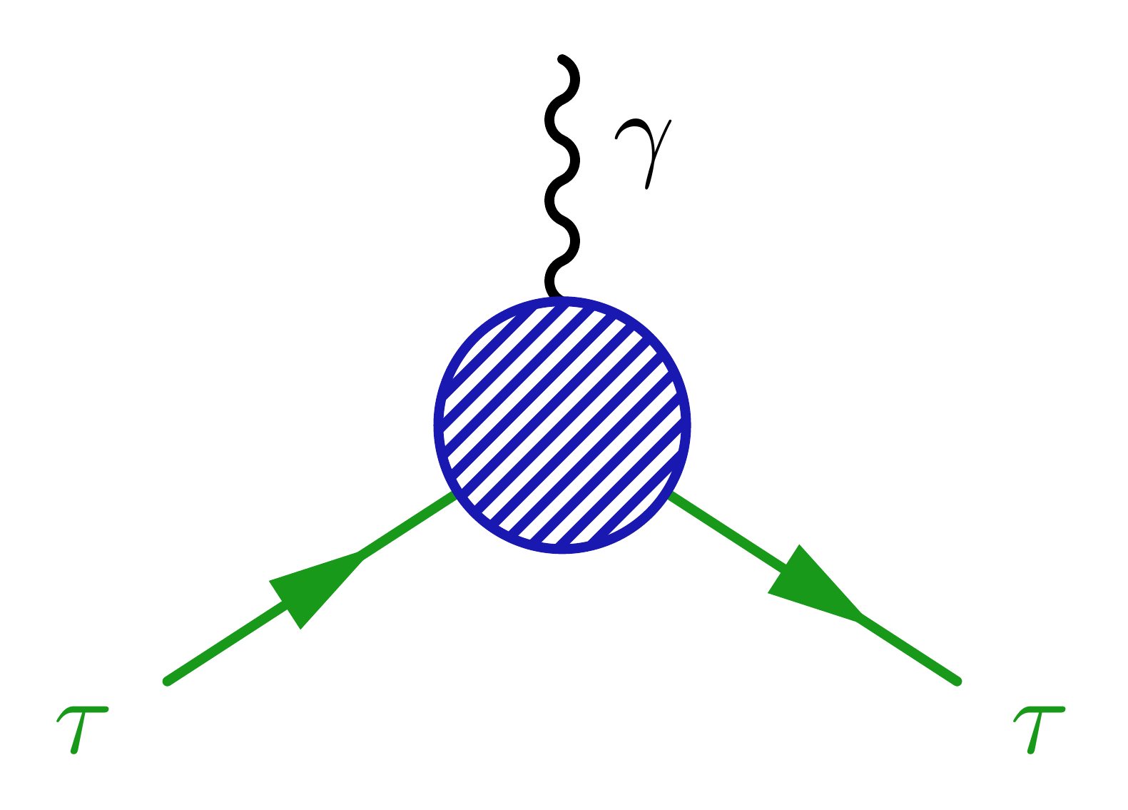
\fmfv{l.a=-50,l.d=8,l=$\gamma$}{g}
\fmfv{l.a=-25,l=\color{collep}$\tau$}{f1}
\fmfv{l.a=-155,l=\color{collep}$\tau$}{f2}
\end{fmfgraph*}
} % close \fmfframe
\end{fmffile}
\end{document}
\documentclass[11pt,border=4pt]{standalone}
\usepackage{feynmp-auto}
\usepackage{xcolor}
\definecolor{collep}{rgb}{.1,.6,.1} % lepton (green)
\definecolor{colvtx}{rgb}{.1,.1,.7} % vertex (dark blue)
\begin{document}
\begin{fmffile}{feyngraph}
  \fmfframe(2,2)(6,2){ % padding (L,T)(R,B)
  \begin{fmfgraph*}(80,85) % canvas (W,H)
    % line style
    \fmfset{wiggly_len}{12} % boson wavelength
    \fmfset{wiggly_slope}{65} % boson slope of waves
    % external vertices
    \fmfbottom{f2,f1}
    \fmftop{g}
    % main process
    \fmf{boson,t=1.2}{g,v} % photon
    \fmf{fermion,f=(.1,,.6,,.1)}{f2,v,f1} % lepton pair
    % labels
    \fmfv{decor.shape=circle,decor.filled=empty,decor.size=35,
       f=(.1,,.1,,.7),b=(.92,,.92,,.98),l=\color{colvtx}$g-2$,l.a=0,l.d=0}{v}
    \fmfv{l.a=-50,l.d=8,l=$\gamma$}{g}
    \fmfv{l.a=-25,l=\color{collep}e}{f1}
    \fmfv{l.a=-155,l=\color{collep}e}{f2}
  \end{fmfgraph*}
  } % close \fmfframe
\end{fmffile}
\end{document}
\documentclass[11pt,border=4pt]{standalone}
\usepackage{feynmp-auto}
\usepackage{xcolor}
\definecolor{collep}{rgb}{.1,.6,.1} % lepton (green)
\definecolor{colvtx}{rgb}{.1,.1,.7} % vertex (dark blue)
\begin{document}
\begin{fmffile}{feyngraph}
  \fmfframe(2,2)(6,2){ % padding (L,T)(R,B)
  \begin{fmfgraph*}(80,85) % canvas (W,H)
    % line style
    \fmfset{wiggly_len}{12} % boson wavelength
    \fmfset{wiggly_slope}{65} % boson slope of waves
    % external vertices
    \fmfbottom{f2,f1}
    \fmftop{g}
    % main process
    \fmf{boson,t=1.2}{g,v} % photon
    \fmf{fermion,f=(.1,,.6,,.1)}{f2,v,f1} % lepton pair
    % labels
    \fmfv{decor.shape=circle,decor.filled=empty,decor.size=35,
       f=(.1,,.1,,.7),b=(.92,,.92,,.98),l=\color{colvtx}$g-2$,l.a=0,l.d=0}{v}
    \fmfv{l.a=-50,l.d=8,l=$\gamma$}{g}
    \fmfv{l.a=-25,l=\color{collep}$\mu$}{f1}
    \fmfv{l.a=-155,l=\color{collep}$\mu$}{f2}
  \end{fmfgraph*}
  } % close \fmfframe
\end{fmffile}
\end{document}
\documentclass[11pt,border=4pt]{standalone}
\usepackage{feynmp-auto}
\usepackage{xcolor}
\definecolor{collep}{rgb}{.1,.6,.1} % lepton (green)
\definecolor{colvtx}{rgb}{.1,.1,.7} % vertex (dark blue)
\begin{document}
\begin{fmffile}{feyngraph}
\fmfframe(2,2)(6,2){ % padding (L,T)(R,B)
\begin{fmfgraph*}(80,85) % canvas (W,H)
% line style
\fmfset{wiggly_len}{12} % boson wavelength
\fmfset{wiggly_slope}{65} % boson slope of waves
% external vertices
\fmfbottom{f2,f1}
\fmftop{g}
% main process
\fmf{boson,t=1.2}{g,v} % photon
\fmf{fermion,f=(.1,,.6,,.1)}{f2,v,f1} % lepton pair
% labels
\fmfv{decor.shape=circle,decor.filled=empty,decor.size=35,
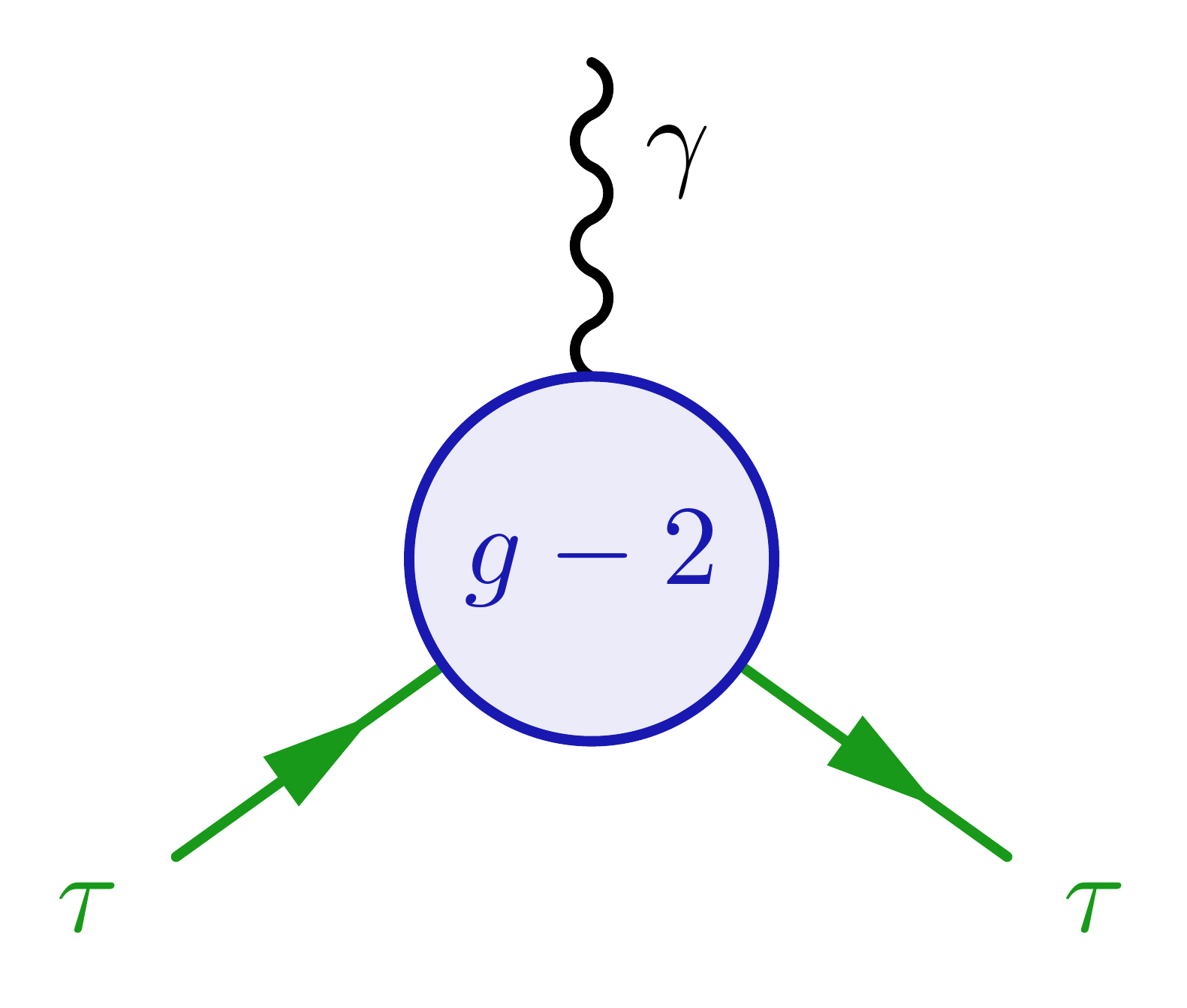
f=(.1,,.1,,.7),b=(.92,,.92,,.98),l=\color{colvtx}$g-2$,l.a=0,l.d=0}{v}
\fmfv{l.a=-50,l.d=8,l=$\gamma$}{g}
\fmfv{l.a=-25,l=\color{collep}$\tau$}{f1}
\fmfv{l.a=-155,l=\color{collep}$\tau$}{f2}
\end{fmfgraph*}
} % close \fmfframe
\end{fmffile}
\end{document}
\documentclass[11pt,border=4pt]{standalone}
\usepackage{feynmp-auto}
\usepackage{xcolor}
\definecolor{collep}{rgb}{.1,.6,.1} % lepton (green)
\definecolor{colvtx}{rgb}{.1,.1,.7} % vertex (dark blue)
\begin{document}
%\begin{fmffile}{feyngraph}
  \fmfframe(2,2)(6,2){ % padding (L,T)(R,B)
%  \begin{fmfgraph*}(90,90) % canvas (W,H)
    % line style
    \fmfset{wiggly_len}{12} % boson wavelength
    \fmfset{wiggly_slope}{65} % boson slope of waves
%    % external vertices
%    \fmfbottom{f2,f1}
%    \fmftop{g}
%    % main process
%    \fmf{boson,t=1.4}{g,v} % photon
%    \fmf{fermion,f=(.1,,.6,,.1)}{f2,v,f1} % lepton pair
%    % labels
%    \fmfv{decor.shape=circle,decor.filled=empty,decor.size=26,
%       f=(.1,,.1,,.7),b=(.92,,.92,,.98),l=\Large\color{colvtx}$g$,l.a=0,l.d=0}{v}
%    \fmfv{l.a=-50,l.d=8,l=$\gamma$}{g}
%    \fmfv{l.a=-25,l=\color{collep}$\lep$}{f1}
%    \fmfv{l.a=-155,l=\color{collep}$\lep$}{f2}
%  \end{fmfgraph*}
%  } % close \fmfframe
\end{fmffile}
\end{document}
\documentclass[11pt,border=4pt]{standalone}
\usepackage{feynmp-auto}
\usepackage{xcolor}
\definecolor{collep}{rgb}{.1,.6,.1} % lepton (green)
\begin{document}
\begin{fmffile}{feyngraph}
  \fmfframe(2,2)(6,2){ % padding (L,T)(R,B)
  \begin{fmfgraph*}(90,90) % canvas (W,H)
    % line style
    \fmfset{wiggly_len}{12} % boson wavelength
    \fmfset{wiggly_slope}{65} % boson slope of waves
    % external vertices
    \fmfbottom{f2,f1}
    \fmftop{g}
    % main process
    \fmf{boson,t=1.2}{g,v} % photon
    \fmf{plain,f=(.1,,.6,,.1),t=1}{v1,v,v2} % internal lepton
    \fmf{fermion,f=(.1,,.6,,.1)}{v1,f1} % incoming lepton
    \fmf{fermion,f=(.1,,.6,,.1)}{f2,v2} % outgoing lepton
    % virtual photon
    \fmffreeze
    \fmf{boson,left=0.3,label=$\gamma$,l.s=left}{v1,v2}
    % labels
    \fmfv{l.a=-50,l.d=8,l=$\gamma$}{g}
    \fmfv{l.a=-25,l=\color{collep}e}{f1}
    \fmfv{l.a=-155,l=\color{collep}e}{f2}
  \end{fmfgraph*}
  } % close \fmfframe
\end{fmffile}
\end{document}
\documentclass[11pt,border=4pt]{standalone}
\usepackage{feynmp-auto}
\usepackage{xcolor}
\definecolor{collep}{rgb}{.1,.6,.1} % lepton (green)
\begin{document}
\begin{fmffile}{feyngraph}
  \fmfframe(2,2)(6,2){ % padding (L,T)(R,B)
  \begin{fmfgraph*}(90,90) % canvas (W,H)
    % line style
    \fmfset{wiggly_len}{12} % boson wavelength
    \fmfset{wiggly_slope}{65} % boson slope of waves
    % external vertices
    \fmfbottom{f2,f1}
    \fmftop{g}
    % main process
    \fmf{boson,t=1.2}{g,v} % photon
    \fmf{plain,f=(.1,,.6,,.1),t=1}{v1,v,v2} % internal lepton
    \fmf{fermion,f=(.1,,.6,,.1)}{v1,f1} % incoming lepton
    \fmf{fermion,f=(.1,,.6,,.1)}{f2,v2} % outgoing lepton
    % virtual photon
    \fmffreeze
    \fmf{boson,left=0.3,label=$\gamma$,l.s=left}{v1,v2}
    % labels
    \fmfv{l.a=-50,l.d=8,l=$\gamma$}{g}
    \fmfv{l.a=-25,l=\color{collep}$\mu$}{f1}
    \fmfv{l.a=-155,l=\color{collep}$\mu$}{f2}
  \end{fmfgraph*}
  } % close \fmfframe
\end{fmffile}
\end{document}
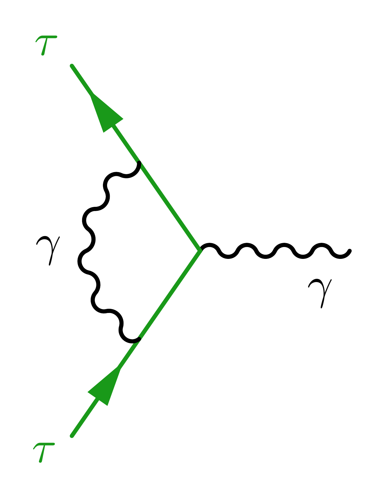
\documentclass[11pt,border=4pt]{standalone}
\usepackage{feynmp-auto}
\usepackage{xcolor}
\definecolor{collep}{rgb}{.1,.6,.1} % lepton (green)
\begin{document}
\begin{fmffile}{feyngraph}
  \fmfframe(2,2)(6,2){ % padding (L,T)(R,B)
  \begin{fmfgraph*}(90,90) % canvas (W,H)
    % line style
    \fmfset{wiggly_len}{12} % boson wavelength
    \fmfset{wiggly_slope}{65} % boson slope of waves
    % external vertices
    \fmfbottom{f2,f1}
    \fmftop{g}
    % main process
    \fmf{boson,t=1.2}{g,v} % photon
    \fmf{plain,f=(.1,,.6,,.1),t=1}{v1,v,v2} % internal lepton
    \fmf{fermion,f=(.1,,.6,,.1)}{v1,f1} % incoming lepton
    \fmf{fermion,f=(.1,,.6,,.1)}{f2,v2} % outgoing lepton
    % virtual photon
    \fmffreeze
    \fmf{boson,left=0.3,label=$\gamma$,l.s=left}{v1,v2}
    % labels
    \fmfv{l.a=-50,l.d=8,l=$\gamma$}{g}
    \fmfv{l.a=-25,l=\color{collep}$\tau$}{f1}
    \fmfv{l.a=-155,l=\color{collep}$\tau$}{f2}
  \end{fmfgraph*}
  } % close \fmfframe
\end{fmffile}
\end{document}
\documentclass[11pt,border=4pt]{standalone}
\usepackage{feynmp-auto}
\usepackage{xcolor}
\definecolor{collep}{rgb}{.1,.6,.1} % lepton (green)
\begin{document}
\begin{fmffile}{feyngraph}
  \fmfframe(2,2)(6,2){ % padding (L,T)(R,B)
  \begin{fmfgraph*}(90,90) % canvas (W,H)
    % line style
    \fmfset{wiggly_len}{12} % boson wavelength
    \fmfset{wiggly_slope}{65} % boson slope of waves
    % external vertices
    \fmfbottom{f2,f1}
    \fmftop{g}
    % main process
    \fmf{boson,t=1.2}{g,v} % photon
    \fmf{plain,f=(.1,,.6,,.1),t=1}{v1,v,v2} % internal lepton
    \fmf{fermion,f=(.1,,.6,,.1)}{v1,f1} % incoming lepton
    \fmf{fermion,f=(.1,,.6,,.1)}{f2,v2} % outgoing lepton
    % virtual photon
    \fmffreeze
    \fmf{boson,label=$\gamma$,l.s=left}{v1,v2}
    % labels
    \fmfv{l.a=-50,l.d=8,l=$\gamma$}{g}
    \fmfv{l.a=-25,l=\color{collep}e}{f1}
    \fmfv{l.a=-155,l=\color{collep}e}{f2}
  \end{fmfgraph*}
  } % close \fmfframe
\end{fmffile}
\end{document}
\documentclass[11pt,border=4pt]{standalone}
\usepackage{feynmp-auto}
\usepackage{xcolor}
\definecolor{collep}{rgb}{.1,.6,.1} % lepton (green)
\begin{document}
\begin{fmffile}{feyngraph}
  \fmfframe(2,2)(6,2){ % padding (L,T)(R,B)
  \begin{fmfgraph*}(90,90) % canvas (W,H)
    % line style
    \fmfset{wiggly_len}{12} % boson wavelength
    \fmfset{wiggly_slope}{65} % boson slope of waves
    % external vertices
    \fmfbottom{f2,f1}
    \fmftop{g}
    % main process
    \fmf{boson,t=1.2}{g,v} % photon
    \fmf{plain,f=(.1,,.6,,.1),t=1}{v1,v,v2} % internal lepton
    \fmf{fermion,f=(.1,,.6,,.1)}{v1,f1} % incoming lepton
    \fmf{fermion,f=(.1,,.6,,.1)}{f2,v2} % outgoing lepton
    % virtual photon
    \fmffreeze
    \fmf{boson,label=$\gamma$,l.s=left}{v1,v2}
    % labels
    \fmfv{l.a=-50,l.d=8,l=$\gamma$}{g}
    \fmfv{l.a=-25,l=\color{collep}$\mu$}{f1}
    \fmfv{l.a=-155,l=\color{collep}$\mu$}{f2}
  \end{fmfgraph*}
  } % close \fmfframe
\end{fmffile}
\end{document}
\documentclass[11pt,border=4pt]{standalone}
\usepackage{feynmp-auto}
\usepackage{xcolor}
\definecolor{collep}{rgb}{.1,.6,.1} % lepton (green)
\begin{document}
\begin{fmffile}{feyngraph}
  \fmfframe(2,2)(6,2){ % padding (L,T)(R,B)
  \begin{fmfgraph*}(90,90) % canvas (W,H)
    % line style
    \fmfset{wiggly_len}{12} % boson wavelength
    \fmfset{wiggly_slope}{65} % boson slope of waves
    % external vertices
    \fmfbottom{f2,f1}
    \fmftop{g}
    % main process
    \fmf{boson,t=1.2}{g,v} % photon
    \fmf{plain,f=(.1,,.6,,.1),t=1}{v1,v,v2} % internal lepton
    \fmf{fermion,f=(.1,,.6,,.1)}{v1,f1} % incoming lepton
    \fmf{fermion,f=(.1,,.6,,.1)}{f2,v2} % outgoing lepton
    % virtual photon
    \fmffreeze
    \fmf{boson,label=$\gamma$,l.s=left}{v1,v2}
    % labels
    \fmfv{l.a=-50,l.d=8,l=$\gamma$}{g}
    \fmfv{l.a=-25,l=\color{collep}$\tau$}{f1}
    \fmfv{l.a=-155,l=\color{collep}$\tau$}{f2}
  \end{fmfgraph*}
  } % close \fmfframe
\end{fmffile}
\end{document}
\documentclass[11pt,border=4pt]{standalone}
\usepackage{feynmp-auto}
\usepackage{xcolor}
\definecolor{collep}{rgb}{.1,.6,.1} % lepton (green)
\begin{document}
\begin{fmffile}{feyngraph}
  \fmfframe(-5,12)(-3,12){ % padding (L,T)(R,B)
  \begin{fmfgraph*}(75,90) % canvas (W,H)
    % line style
    \fmfset{wiggly_len}{12} % boson wavelength
    \fmfset{wiggly_slope}{65} % boson slope of waves
    % external vertices
    \fmfright{g}
    \fmfleft{f2,f1}
    % main process
    \fmf{boson,t=0.9}{g,v} % photon
    \fmf{plain,f=(.1,,.6,,.1),t=1.1}{v1,v,v2} % internal lepton
    \fmf{fermion,f=(.1,,.6,,.1)}{v1,f1} % incoming lepton
    \fmf{fermion,f=(.1,,.6,,.1)}{f2,v2} % outgoing lepton
    % virtual photon
    \fmffreeze
    \fmf{boson,right=0.6,label=$\gamma$,l.s=right}{v1,v2}
    % labels
    \fmfv{l.a=-120,l.d=8,l=$\gamma$}{g}
    \fmfv{l.a=140,l.d=4,l=\color{collep}e}{f1}
    \fmfv{l.a=-155,l.d=4,l=\color{collep}e}{f2}
  \end{fmfgraph*}
  } % close \fmfframe
\end{fmffile}
\end{document}
\documentclass[11pt,border=4pt]{standalone}
\usepackage{feynmp-auto}
\usepackage{xcolor}
\definecolor{collep}{rgb}{.1,.6,.1} % lepton (green)
\begin{document}
\begin{fmffile}{feyngraph}
  \fmfframe(-5,12)(-3,12){ % padding (L,T)(R,B)
  \begin{fmfgraph*}(75,90) % canvas (W,H)
    % line style
    \fmfset{wiggly_len}{12} % boson wavelength
    \fmfset{wiggly_slope}{65} % boson slope of waves
    % external vertices
    \fmfright{g}
    \fmfleft{f2,f1}
    % main process
    \fmf{boson,t=0.9}{g,v} % photon
    \fmf{plain,f=(.1,,.6,,.1),t=1.1}{v1,v,v2} % internal lepton
    \fmf{fermion,f=(.1,,.6,,.1)}{v1,f1} % incoming lepton
    \fmf{fermion,f=(.1,,.6,,.1)}{f2,v2} % outgoing lepton
    % virtual photon
    \fmffreeze
    \fmf{boson,right=0.6,label=$\gamma$,l.s=right}{v1,v2}
    % labels
    \fmfv{l.a=-120,l.d=8,l=$\gamma$}{g}
    \fmfv{l.a=140,l.d=4,l=\color{collep}$\mu$}{f1}
    \fmfv{l.a=-155,l.d=4,l=\color{collep}$\mu$}{f2}
  \end{fmfgraph*}
  } % close \fmfframe
\end{fmffile}
\end{document}
Full code
The LaTeX code below collects all the diagrams above into one big file that produces a multipage PDF. Please find download links below, or edit and compile here if you like:
% !TEX program = pdflatexmk
% !TEX parameter = -shell-escape
% Author: Izaak Neutelings (February 2024)
% Description: Anomalous magnetic moment in pp collisions
% Sources: https://cms.cern.ch/iCMS/analysisadmin/cadilines?line=EXO-23-005
% Instructions: To compile via command line, run the following twice
%   pdflatex -shell-escape anomalous_momentum_pp.tex
\documentclass[11pt,border=4pt,multi=page,crop]{standalone}
\usepackage{feynmp-auto}
\usepackage{xcolor}
\usepackage{pgffor} % for \foreach

% DEFINE TEXT COLORS
\definecolor{collep}{rgb}{.1,.6,.1} % lepton (green)
\definecolor{colvtx}{rgb}{.1,.1,.7} % vertex (dark blue)

% DEFINE COLOR MACROS
% The following loops over the user color names and defines
% a handy \<colname> command to set text color, as well as
% defines colors in MetaPost of the same and value for lines
\usepackage{pgffor} % for \foreach
\def\MPcolors{} % MetaPost code importing xcolor names
\foreach \colname in {collep,colvtx}{ % create command & MetaPost code
  \expandafter\xdef\csname\colname\endcsname{\noexpand\color{\colname}}% \newcommand\<colname>
  \convertcolorspec{named}{\colname}{rgb}\tmprgb % get rgb code
  \xdef\MPcolors{\MPcolors color \colname; \colname := (\tmprgb); } % add color name
}

% DEFINE fmfpicture ENVIRONMENT
% The following defines a custom picture environment that
% helps to create standalone pages with common settings,
% and correctly padding the diagram with \fmfframe
\usepackage{environ} % for \NewEnviron
\NewEnviron{fmfpicture}[3]{%
  \begin{page} % to create standalone page
  \fmfframe(#1)(#2){ % padding (LT)(RB)
  \begin{fmffile}{feynmp-#3} % auxiliary files (use unique name!)
    \fmfset{wiggly_len}{12} % boson wavelength
    \fmfset{wiggly_slope}{65} % boson slope of waves
    \fmfcmd\MPcolors % define custom line colors in MetaPost (does not work in \fmfv)
    \BODY % main code
  \end{fmffile}
  }
  \end{page}
}

% LOOP MACRO
%\def\foreachlep#1{\foreach \lep in {\ell,\tau}{#1}}
\def\foreachlep#1{\foreach \lep in {\mathrm{e},\mu,\tau}{#1}}
%\def\foreachlep#1{\foreach \lep in {\mathrm{e},\mu,\tau,\ell}{#1}}

\begin{document}


% gamma -> tautau LO, color
\foreachlep{ % loop over leptons labels
\begin{fmfpicture}{2,2}{6,2}{v-gamma-tautau-lo} % padding (LT)(RB)
  \begin{fmfgraph*}(80,70) % canvas (W,H)
    % external vertices
    \fmfbottom{f2,f1}
    \fmftop{g}
    % main process
    \fmf{boson,t=1.4}{g,v} % photon
    \fmf{fermion,f=collep}{f2,v,f1} % lepton pair
    % labels
    \fmfv{l.a=-50,l.d=8,l=$\gamma$}{g}
    \fmfv{l.a=-25,l=\collep$\lep$}{f1}
    \fmfv{l.a=-155,l=\collep$\lep$}{f2}
  \end{fmfgraph*}
\end{fmfpicture}
} % close \foreach loop


% gamma -> tautau blob (g-2)
\foreachlep{ % loop over leptons labels
\begin{fmfpicture}{2,2}{6,2}{v-gamma-tautau-blob} % padding (LT)(RB)
  \begin{fmfgraph*}(80,70) % canvas (W,H)
    % external vertices
    \fmfbottom{f2,f1}
    \fmftop{g}
    % main process
    \fmf{boson,t=1.4}{g,v} % photon
    \fmf{fermion,f=collep}{f2,v,f1} % lepton pair
    % labels
    \fmfv{d.s=circle,d.s=4,f=colvtx,d.f=full}{v} %,l.d=12,l.a=0,
          %l=\normalsize\colvtx$C_{\tau B}/\Lambda^2$}{vt}
    \fmfblob{25}{v} % use \fmfv first to give color
    \fmfv{l.a=-50,l.d=8,l=$\gamma$}{g}
    \fmfv{l.a=-25,l=\collep$\lep$}{f1}
    \fmfv{l.a=-155,l=\collep$\lep$}{f2}
  \end{fmfgraph*}
\end{fmfpicture}
} % close \foreach loop


% gamma -> tautau blob (g-2)
\foreachlep{ % loop over leptons labels
\begin{fmfpicture}{2,2}{6,2}{v-gamma-tautau-blob-label2} % padding (LT)(RB)
  \begin{fmfgraph*}(80,85) % canvas (W,H)
    % external vertices
    \fmfbottom{f2,f1}
    \fmftop{g}
    % main process
    \fmf{boson,t=1.2}{g,v} % photon
    \fmf{fermion,f=collep}{f2,v,f1} % lepton pair
    % labels
    \fmfv{decor.shape=circle,decor.filled=empty,decor.size=35,
       f=colvtx,b=(.92,,.92,,.98),l=\colvtx$g-2$,l.a=0,l.d=0}{v}
    \fmfv{l.a=-50,l.d=8,l=$\gamma$}{g}
    \fmfv{l.a=-25,l=\collep$\lep$}{f1}
    \fmfv{l.a=-155,l=\collep$\lep$}{f2}
  \end{fmfgraph*}
\end{fmfpicture}
} % close \foreach loop


%% gamma -> tautau blob (g-2)
%\foreachlep{ % loop over leptons labels
%\begin{fmfpicture}{2,2}{6,2}{v-gamma-tautau-blob-label} % padding (LT)(RB)
%  \begin{fmfgraph*}(90,90) % canvas (W,H)
%    % external vertices
%    \fmfbottom{f2,f1}
%    \fmftop{g}
%    % main process
%    \fmf{boson,t=1.4}{g,v} % photon
%    \fmf{fermion,f=collep}{f2,v,f1} % lepton pair
%    % labels
%    \fmfv{decor.shape=circle,decor.filled=empty,decor.size=26,
%       f=colvtx,b=(.92,,.92,,.98),l=\Large\colvtx$g$,l.a=0,l.d=0}{v}
%    \fmfv{l.a=-50,l.d=8,l=$\gamma$}{g}
%    \fmfv{l.a=-25,l=\collep$\lep$}{f1}
%    \fmfv{l.a=-155,l=\collep$\lep$}{f2}
%  \end{fmfgraph*}
%\end{fmfpicture}
%} % close \foreach loop


% gamma -> tautau round loop (g-2)
\foreachlep{ % loop over leptons labels
\begin{fmfpicture}{2,2}{6,2}{v-gamma-tautau-loop} % padding (LT)(RB)
  \begin{fmfgraph*}(90,90) % canvas (W,H)
    % external vertices
    \fmfbottom{f2,f1}
    \fmftop{g}
    % main process
    \fmf{boson,t=1.2}{g,v} % photon
    \fmf{plain,f=collep,t=1}{v1,v,v2} % internal lepton
    \fmf{fermion,f=collep}{v1,f1} % incoming lepton
    \fmf{fermion,f=collep}{f2,v2} % outgoing lepton
    % virtual photon
    \fmffreeze
    \fmf{boson,left=0.3,label=$\gamma$,l.s=left}{v1,v2}
    % labels
    \fmfv{l.a=-50,l.d=8,l=$\gamma$}{g}
    \fmfv{l.a=-25,l=\collep$\lep$}{f1}
    \fmfv{l.a=-155,l=\collep$\lep$}{f2}
  \end{fmfgraph*}
\end{fmfpicture}
} % close \foreach loop


% gamma -> tautau straight loop (g-2)
\foreachlep{ % loop over leptons labels
\begin{fmfpicture}{2,2}{6,2}{v-gamma-tautau-loop-straight} % padding (LT)(RB)
  \begin{fmfgraph*}(90,90) % canvas (W,H)
    % external vertices
    \fmfbottom{f2,f1}
    \fmftop{g}
    % main process
    \fmf{boson,t=1.2}{g,v} % photon
    \fmf{plain,f=collep,t=1}{v1,v,v2} % internal lepton
    \fmf{fermion,f=collep}{v1,f1} % incoming lepton
    \fmf{fermion,f=collep}{f2,v2} % outgoing lepton
    % virtual photon
    \fmffreeze
    \fmf{boson,label=$\gamma$,l.s=left}{v1,v2}
    % labels
    \fmfv{l.a=-50,l.d=8,l=$\gamma$}{g}
    \fmfv{l.a=-25,l=\collep$\lep$}{f1}
    \fmfv{l.a=-155,l=\collep$\lep$}{f2}
  \end{fmfgraph*}
\end{fmfpicture}
} % close \foreach loop


% gamma -> tautau round loop vertical (g-2)
\foreachlep{ % loop over leptons labels
\begin{fmfpicture}{-5,12}{-3,12}{v-gamma-tautau-loop-left} % padding (LT)(RB)
  \begin{fmfgraph*}(75,90) % canvas (W,H)
    % external vertices
    \fmfright{g}
    \fmfleft{f2,f1}
    % main process
    \fmf{boson,t=0.9}{g,v} % photon
    \fmf{plain,f=collep,t=1.1}{v1,v,v2} % internal lepton
    \fmf{fermion,f=collep}{v1,f1} % incoming lepton
    \fmf{fermion,f=collep}{f2,v2} % outgoing lepton
    % virtual photon
    \fmffreeze
    \fmf{boson,right=0.6,label=$\gamma$,l.s=right}{v1,v2}
    % labels
    \fmfv{l.a=-120,l.d=8,l=$\gamma$}{g}
    \fmfv{l.a=140,l.d=4,l=\collep$\lep$}{f1}
    \fmfv{l.a=-155,l.d=4,l=\collep$\lep$}{f2}
  \end{fmfgraph*}
\end{fmfpicture}
} % close \foreach loop


\end{document}
Click to download: g-2.tex • g-2.pdf
Open in Overleaf: g-2.tex
")
")