This posts shows code examples of Feynman diagrams of top quark pair production in association with charm quarks in proton-proton collisions. The charm quarks are highlighted with orange jet cones, inspired by the diagrams in this publication on the search for this process at ATLAS. The same search was performed at CMS. For a nice talk on the search for H → cc decay in ttH production at the LHC, where this ttcc is a large background, see this recorded CERN seminar by Sebastian Wuchterl.
Click on a diagram to jump to the code & download links below: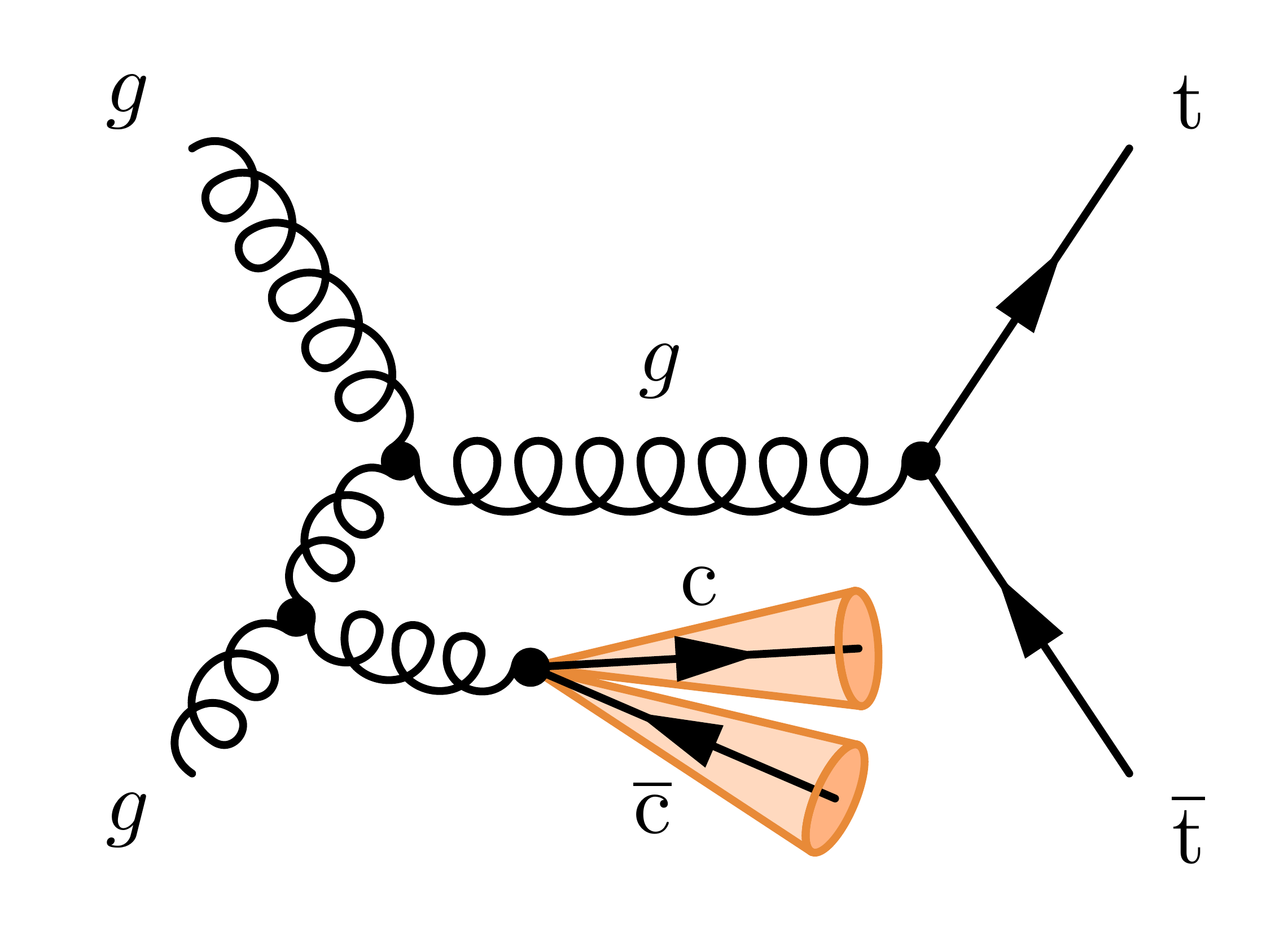
ttcc production via initial-state gluon radiation, where the charm jets are resolved:
\documentclass[11pt,border=4pt]{standalone}
\usepackage{feynmp-auto}

% HELP MACRO to create convert numbers to letters
% This is needed because MetaPost cannot handle variable names with numbers
\makeatletter
  \newcommand{\numberToRoman}[1]{\@Roman{#1}}
\makeatother

% JET CONE MACRO
\def\ijc{0} % start \ijc counter from 0
\def\fmfcone[a=#1,e=#2,s=#3]#4#5{
  % Create a 3D-like jet cone between two given vertices
  % The computations for tangents to an ellipse are based on
  %   https://tikz.net/circle_tangent/
  % Arguments:
  %   a = half of cone's opening angle (degrees), e.g. 20
  %   e = excentricity as ratio rx/ry, e.g. 0.15
  %   s = length to shorten or elongate cone
  %   #4, #5 = vertices defining the direction
  \fmffreeze % needed to access vertices in MetaPost
  \edef\ijc{\number\numexpr\ijc + 1\relax} % increment \ijc counter
  \edef\jcpath{conebase_\numberToRoman{\ijc}} % add space
  \message{^^J^^J  path name=\jcpath\ for \ijc=\ijc}
  \edef\tmpcmd{% expand macros inside \fmfcmd before executing it
    \noexpand\fmfcmd{ % draw behind Feynman diagram
      % settings
      pair A, B, C, O;
      numeric ang; ang := #1; % half of cone's opening angle
      numeric e; e := #2; % excentricity as ratio rx/ry
      message "  fmfcone \jcpath: e=" & decimal(e) & ", ang=" & decimal(ang);
      % vector
      A := vloc(__#4); % vertex origin
      O := vloc(__#5); % center of ellipse
      numeric len_jc; len_jc := length(O-A); % distance between A and B
      numeric ang_jc; ang_jc := angle(O-A);
      O := O + (#3,0) rotated ang_jc; % add shift
      message "  fmfcone \jcpath: len_jc=" & decimal(len_jc) & ", ang_jc=" & decimal(ang_jc);
      % tangents to ellipse
      x := len_jc*e*sind(ang)*sind(ang); % x coordinate P
      y := (len_jc-x)*sind(ang)/cosd(ang); % y coordinate P
      B := O + (-x, y) rotated ang_jc; % tangent point 1
      C := O + (-x,-y) rotated ang_jc; % tangent point 2
      message "  fmfcone \jcpath: x=" & decimal(x) & ", y=" & decimal(y);
      % triangle
      path cone; cone := A -- B -- C -- cycle;
      fill cone withcolor coljetfill;
      draw cone withcolor coljetline;
      % ellipse base
      numeric rx, ry;
      rx := len_jc*sqrt(e)*sind(ang); % horizontal radius
      ry := len_jc*sind(ang)/cosd(ang)*sqrt(1-e*sind(ang)*sind(ang)); % vertical radius
      message "  fmfcone \jcpath: rx=" & decimal(rx) & ", ry=" & decimal(ry);
      path \jcpath;
      \jcpath := fullcircle xscaled (2*rx) yscaled (2*ry) rotated ang_jc shifted O;
      fill \jcpath\ withcolor coljetbase;
      draw \jcpath\ withcolor coljetline;
      % custom line style to draw on top
      style_def jet\jcpath\ expr p =
        draw subpath (2,6) of \jcpath\ withcolor coljetline;
      enddef;
    } % end \fmfcmd
    \noexpand\fmf{jet\jcpath}{#4,#4_#5_help_,#5} % draw are in front of Feynman diagram
  }\tmpcmd % execute above lines now that all macros are expanded
}

\begin{document}
\begin{fmffile}{feyngraph}
  \fmfframe(-7,17)(-4,18){ % padding (L,T)(R,B)
  \begin{fmfgraph*}(150,80) % dimensions (WH)
    % line style
    \fmfset{dash_len}{10} % dashes length
    \fmfset{wiggly_len}{12} % boson wavelength
    \fmfset{wiggly_slope}{65} % boson slope of waves
    % line colors
    \fmfcmd{
      color coljetline; coljetline := (.91,.54,.22); % jet line color
      color coljetfill; coljetfill := (1.0,.85,.75); % jet fill color
      color coljetbase; coljetbase := (1.0,.70,.50); % jet base fill color
    }
    % external vertices
    \fmfleft{i2,i1}
    \fmfright{o2,o1}
    % main
    \fmf{gluon}{v1,i1}
    \fmf{gluon,t=2}{v1,vr,i2}
    \fmf{fermion}{o2,v2,o1}
    \fmf{gluon,tension=0.8,label=$g$,label.side=left,label.dist=8}{v1,v2} % s-channel
    \fmfdot{v1,v2,vr,vcc}
    % initial-state radiation
    \fmffreeze
    \fmfforce{vloc(__vr)+(.2w,-.08h)}{vcc} % exact placement
    \fmfforce{vloc(__vcc)+(.28w,.03h)}{c1} % exact placement
    \fmfforce{vloc(__vcc)+(.26w,-.21h)}{c2} % exact placement
    \fmf{gluon}{vr,vcc} % gluon radiation
    \fmf{fermion,l.d=6.7,l.s=left,label=c}{vcc,c1} % charm 1
    \fmf{fermion,l.d=6,l.s=left,label=$\overline{\mathrm{c}}$}{c2,vcc} % charm 2
    %\fmfcmd{coljetline := red;} % override default color
    \fmfcone[a=10,e=0.12,s=0]{vcc}{c1} % jet cone
    \fmfcone[a=10,e=0.12,s=0]{vcc}{c2} % jet cone
    % labels
    \fmfv{l.a=155,l.d=6,l=$g$}{i1}
    \fmfv{l.a=-155,l.d=6,l=$g$}{i2}
    \fmfv{l.a=25,l.d=6,l=t}{o1}
    \fmfv{l.a=-25,l.d=6,l=$\overline{\mathrm{t}}$}{o2}
  \end{fmfgraph*}
  } % close \fmfframe
\end{fmffile}
\end{document}
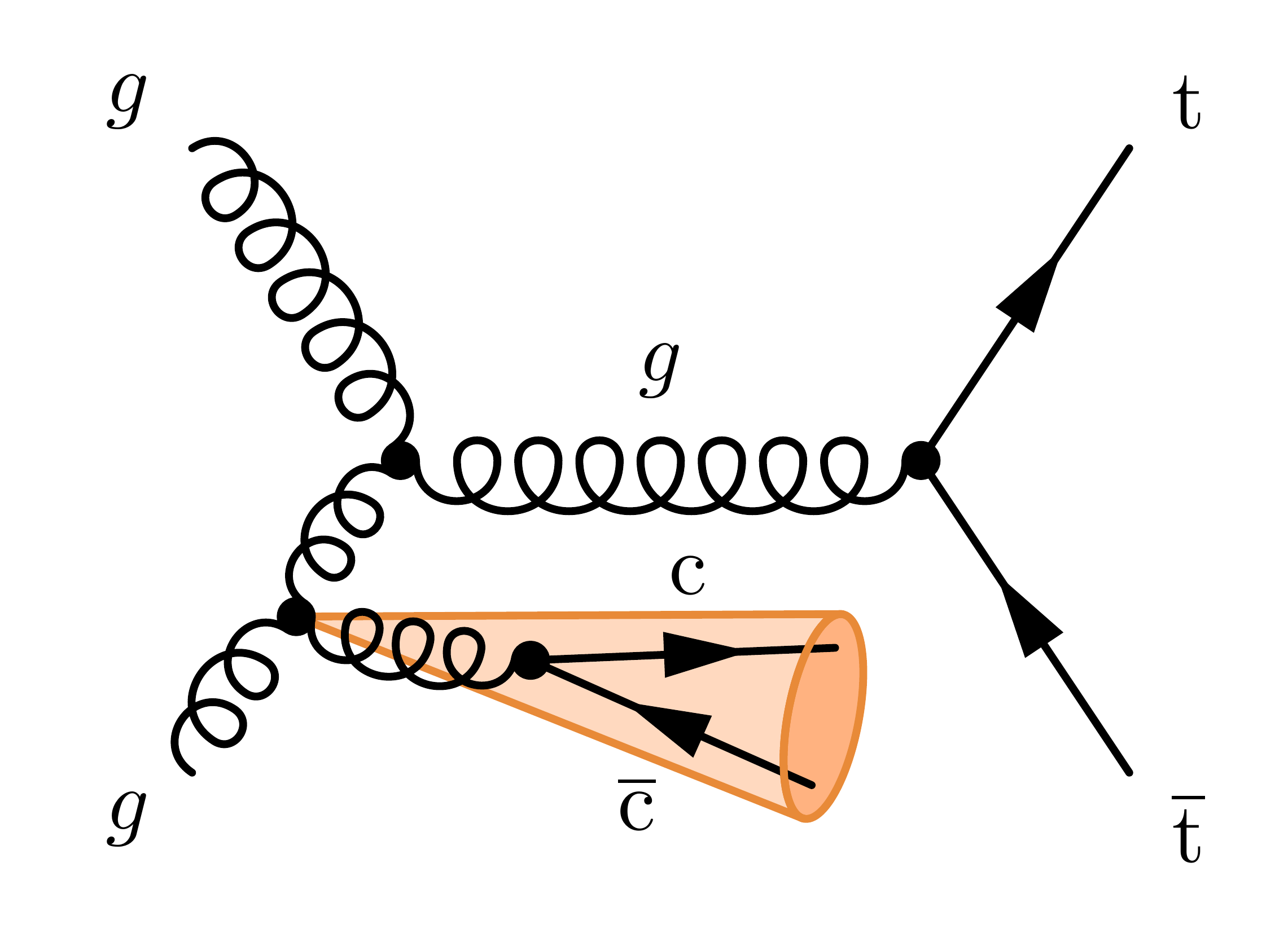
ttcc productionvia initial-state gluon radiation, where the charm jets are merged:
\documentclass[11pt,border=4pt]{standalone}
\usepackage{feynmp-auto}

% HELP MACRO to create convert numbers to letters
% This is needed because MetaPost cannot handle variable names with numbers
\makeatletter
  \newcommand{\numberToRoman}[1]{\@Roman{#1}}
\makeatother

% JET CONE MACRO
\def\ijc{0} % start \ijc counter from 0
\def\fmfcone[a=#1,e=#2,s=#3]#4#5{
  % Create a 3D-like jet cone between two given vertices
  % The computations for tangents to an ellipse are based on
  %   https://tikz.net/circle_tangent/
  % Arguments:
  %   a = half of cone's opening angle (degrees), e.g. 20
  %   e = excentricity as ratio rx/ry, e.g. 0.15
  %   s = length to shorten or elongate cone
  %   #4, #5 = vertices defining the direction
  \fmffreeze % needed to access vertices in MetaPost
  \edef\ijc{\number\numexpr\ijc + 1\relax} % increment \ijc counter
  \edef\jcpath{conebase_\numberToRoman{\ijc}} % add space
  \message{^^J^^J  path name=\jcpath\ for \ijc=\ijc}
  \edef\tmpcmd{% expand macros inside \fmfcmd before executing it
    \noexpand\fmfcmd{ % draw behind Feynman diagram
      % settings
      pair A, B, C, O;
      numeric ang; ang := #1; % half of cone's opening angle
      numeric e; e := #2; % excentricity as ratio rx/ry
      message "  fmfcone \jcpath: e=" & decimal(e) & ", ang=" & decimal(ang);
      % vector
      A := vloc(__#4); % vertex origin
      O := vloc(__#5); % center of ellipse
      numeric len_jc; len_jc := length(O-A); % distance between A and B
      numeric ang_jc; ang_jc := angle(O-A);
      O := O + (#3,0) rotated ang_jc; % add shift
      message "  fmfcone \jcpath: len_jc=" & decimal(len_jc) & ", ang_jc=" & decimal(ang_jc);
      % tangents to ellipse
      x := len_jc*e*sind(ang)*sind(ang); % x coordinate P
      y := (len_jc-x)*sind(ang)/cosd(ang); % y coordinate P
      B := O + (-x, y) rotated ang_jc; % tangent point 1
      C := O + (-x,-y) rotated ang_jc; % tangent point 2
      message "  fmfcone \jcpath: x=" & decimal(x) & ", y=" & decimal(y);
      % triangle
      path cone; cone := A -- B -- C -- cycle;
      fill cone withcolor coljetfill;
      draw cone withcolor coljetline;
      % ellipse base
      numeric rx, ry;
      rx := len_jc*sqrt(e)*sind(ang); % horizontal radius
      ry := len_jc*sind(ang)/cosd(ang)*sqrt(1-e*sind(ang)*sind(ang)); % vertical radius
      message "  fmfcone \jcpath: rx=" & decimal(rx) & ", ry=" & decimal(ry);
      path \jcpath;
      \jcpath := fullcircle xscaled (2*rx) yscaled (2*ry) rotated ang_jc shifted O;
      fill \jcpath\ withcolor coljetbase;
      draw \jcpath\ withcolor coljetline;
      % custom line style to draw on top
      style_def jet\jcpath\ expr p =
        draw subpath (2,6) of \jcpath\ withcolor coljetline;
      enddef;
    } % end \fmfcmd
    \noexpand\fmf{jet\jcpath}{#4,#4_#5_help_,#5} % draw are in front of Feynman diagram
  }\tmpcmd % execute above lines now that all macros are expanded
}

\begin{document}
\begin{fmffile}{feyngraph}
  \fmfframe(-7,17)(-4,18){ % padding (L,T)(R,B)
  \begin{fmfgraph*}(150,80) % dimensions (WH)
    % line style
    \fmfset{dash_len}{10} % dashes length
    \fmfset{wiggly_len}{12} % boson wavelength
    \fmfset{wiggly_slope}{65} % boson slope of waves
    % line colors
    \fmfcmd{
      color coljetline; coljetline := (.91,.54,.22); % jet line color
      color coljetfill; coljetfill := (1.0,.85,.75); % jet fill color
      color coljetbase; coljetbase := (1.0,.70,.50); % jet base fill color
    }
    % external vertices
    \fmfleft{i2,i1}
    \fmfright{o2,o1}
    % main
    \fmf{gluon}{v1,i1}
    \fmf{gluon,t=2}{v1,vr,i2}
    \fmf{fermion}{o2,v2,o1}
    \fmf{gluon,tension=0.8,label=$g$,label.side=left,label.dist=8}{v1,v2} % s-channel
    \fmfdot{v1,v2,vr,vcc}
    % initial-state radiation
    \fmffreeze
    \fmfforce{vloc(__vr)+(.2w,-.07h)}{vcc} % exact placement
    \fmfforce{vloc(__vcc)+(.26w,.02h)}{c1} % exact placement
    \fmfforce{vloc(__vcc)+(.24w,-.20h)}{c2} % exact placement
    \fmfforce{0.5*(vloc(__c1)+vloc(__c2))}{c} % exact placement
    \fmf{gluon}{vr,vcc} % gluon radiation
    \fmf{fermion,l.d=7.6,l.s=left,label=c}{vcc,c1} % charm 1
    \fmf{fermion,l.d=7,l.s=left,label=$\overline{\mathrm{c}}$}{c2,vcc} % charm 2
    %\fmfcmd{coljetline := red;} % override default color
    \fmfcone[a=11,e=0.12,s=0]{vr}{c} % jet cone
    % labels
    \fmfv{l.a=155,l.d=6,l=$g$}{i1}
    \fmfv{l.a=-155,l.d=6,l=$g$}{i2}
    \fmfv{l.a=25,l.d=6,l=t}{o1}
    \fmfv{l.a=-25,l.d=6,l=$\overline{\mathrm{t}}$}{o2}
  \end{fmfgraph*}
  } % close \fmfframe
\end{fmffile}
\end{document}
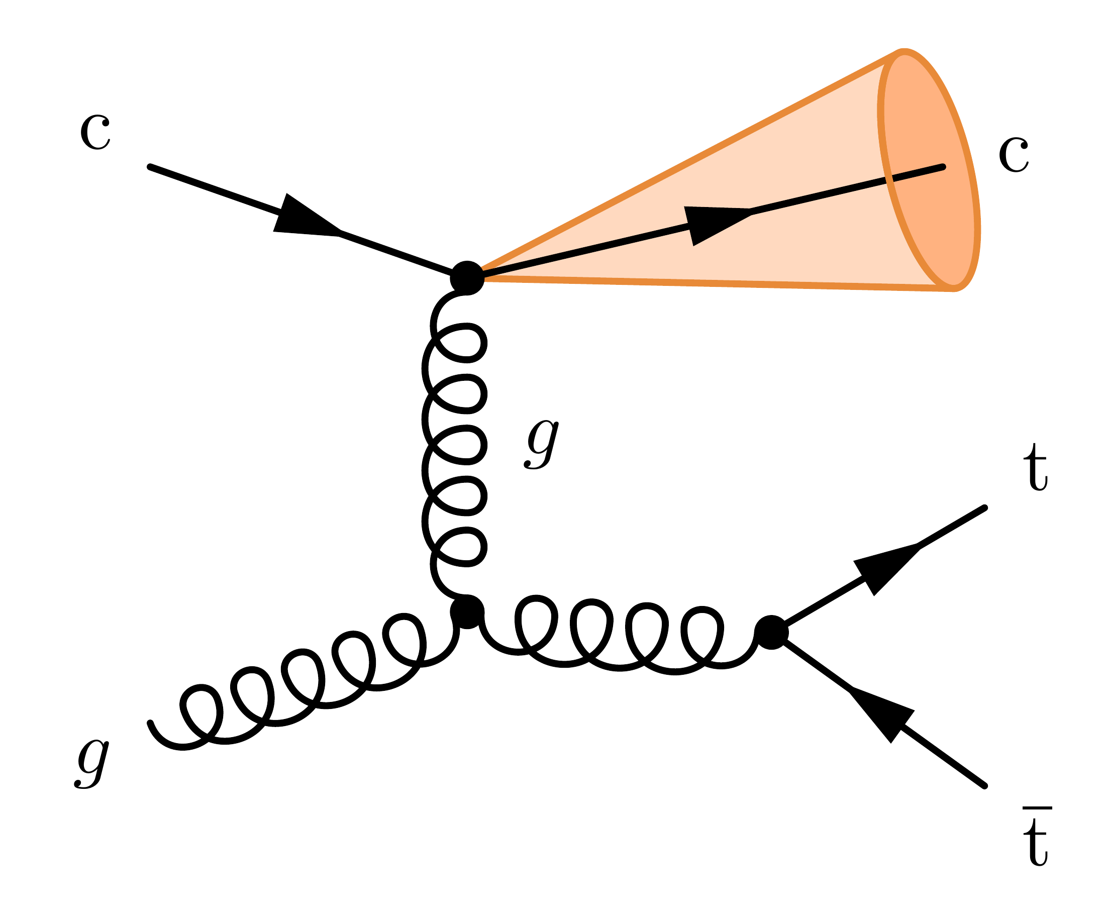
ttc production, where the charm quark originates from the initial state:
\documentclass[11pt,border=4pt]{standalone}
\usepackage{feynmp-auto}

% HELP MACRO to create convert numbers to letters
% This is needed because MetaPost cannot handle variable names with numbers
\makeatletter
  \newcommand{\numberToRoman}[1]{\@Roman{#1}}
\makeatother

% JET CONE MACRO
\def\ijc{0} % start \ijc counter from 0
\def\fmfcone[a=#1,e=#2,s=#3]#4#5{
  % Create a 3D-like jet cone between two given vertices
  % The computations for tangents to an ellipse are based on
  %   https://tikz.net/circle_tangent/
  % Arguments:
  %   a = half of cone's opening angle (degrees), e.g. 20
  %   e = excentricity as ratio rx/ry, e.g. 0.15
  %   s = length to shorten or elongate cone
  %   #4, #5 = vertices defining the direction
  \fmffreeze % needed to access vertices in MetaPost
  \edef\ijc{\number\numexpr\ijc + 1\relax} % increment \ijc counter
  \edef\jcpath{conebase_\numberToRoman{\ijc}} % add space
  \message{^^J^^J  path name=\jcpath\ for \ijc=\ijc}
  \edef\tmpcmd{% expand macros inside \fmfcmd before executing it
    \noexpand\fmfcmd{ % draw behind Feynman diagram
      % settings
      pair A, B, C, O;
      numeric ang; ang := #1; % half of cone's opening angle
      numeric e; e := #2; % excentricity as ratio rx/ry
      message "  fmfcone \jcpath: e=" & decimal(e) & ", ang=" & decimal(ang);
      % vector
      A := vloc(__#4); % vertex origin
      O := vloc(__#5); % center of ellipse
      numeric len_jc; len_jc := length(O-A); % distance between A and B
      numeric ang_jc; ang_jc := angle(O-A);
      O := O + (#3,0) rotated ang_jc; % add shift
      message "  fmfcone \jcpath: len_jc=" & decimal(len_jc) & ", ang_jc=" & decimal(ang_jc);
      % tangents to ellipse
      x := len_jc*e*sind(ang)*sind(ang); % x coordinate P
      y := (len_jc-x)*sind(ang)/cosd(ang); % y coordinate P
      B := O + (-x, y) rotated ang_jc; % tangent point 1
      C := O + (-x,-y) rotated ang_jc; % tangent point 2
      message "  fmfcone \jcpath: x=" & decimal(x) & ", y=" & decimal(y);
      % triangle
      path cone; cone := A -- B -- C -- cycle;
      fill cone withcolor coljetfill;
      draw cone withcolor coljetline;
      % ellipse base
      numeric rx, ry;
      rx := len_jc*sqrt(e)*sind(ang); % horizontal radius
      ry := len_jc*sind(ang)/cosd(ang)*sqrt(1-e*sind(ang)*sind(ang)); % vertical radius
      message "  fmfcone \jcpath: rx=" & decimal(rx) & ", ry=" & decimal(ry);
      path \jcpath;
      \jcpath := fullcircle xscaled (2*rx) yscaled (2*ry) rotated ang_jc shifted O;
      fill \jcpath\ withcolor coljetbase;
      draw \jcpath\ withcolor coljetline;
      % custom line style to draw on top
      style_def jet\jcpath\ expr p =
        draw subpath (2,6) of \jcpath\ withcolor coljetline;
      enddef;
    } % end \fmfcmd
    \noexpand\fmf{jet\jcpath}{#4,#4_#5_help_,#5} % draw are in front of Feynman diagram
  }\tmpcmd % execute above lines now that all macros are expanded
}

\begin{document}
\begin{fmffile}{feyngraph}
  \fmfframe(5,22)(8,26){ % padding (L,T)(R,B)
  \begin{fmfgraph*}(120,80) % dimensions (WH)
    % line style
    \fmfset{dash_len}{10} % dashes length
    \fmfset{wiggly_len}{12} % boson wavelength
    \fmfset{wiggly_slope}{65} % boson slope of waves
    % line colors
    \fmfcmd{
      color coljetline; coljetline := (.91,.54,.22); % jet line color
      color coljetfill; coljetfill := (1.0,.85,.75); % jet fill color
      color coljetbase; coljetbase := (1.0,.70,.50); % jet base fill color
    }
    % external vertices
    \fmfstraight
    \fmfleft{i2,i1}
    \fmfright{o3,o2,o1}
    \fmfshift{6 left}{o1}
    \fmfshift{9 down}{o2,o3}
    \fmfforce{(.38w,.8h)}{v1} % exact placement
    \fmfforce{(.38w,.2h)}{v2} % exact placement
    % main
    \fmf{quark}{i1,v1}
    \fmf{gluon}{i2,v2}
    \fmf{fermion}{v1,o1}
    \fmf{gluon,tension=0.8,label=$g$,label.side=left,label.dist=8}{v1,v2} % t-channel
    \fmfdot{v1,v2,vtt}
    % ttbar
    \fmf{gluon,t=1.4}{v2,vtt}
    \fmf{fermion}{o3,vtt,o2}
    % initial-state radiation
    %\fmfcmd{coljetline := red;} % override default color
    \fmfcone[a=14,e=0.12,s=-2]{v1}{o1} % jet cone
    % labels
    \fmfv{l.a=155,l.d=6,l=c}{i1}
    \fmfv{l.a=-155,l.d=6,l=$g$}{i2}
    \fmfv{l.a=12,l.d=8,l=c}{o1}
    \fmfv{l.a=25,l.d=6,l=t}{o2}
    \fmfv{l.a=-25,l.d=6,l=$\overline{\mathrm{t}}$}{o3}
  \end{fmfgraph*}
  } % close \fmfframe
\end{fmffile}
\end{document}
Full code
The LaTeX code below collects all the diagrams above into one big file that produces a multipage PDF. Please find download links below, or edit and compile here if you like:
% !TEX program = pdflatexmk
% !TEX parameter = -shell-escape
% Author: Izaak Neutelings (June 2024)
% Sources:
%   https://twiki.cern.ch/twiki/bin/view/LHCPhysics/CrossSections
% Instructions: To compile via command line, run the following twice
%   pdflatex -shell-escape higgs_pp.tex
\documentclass[11pt,border=4pt,multi=page,crop]{standalone}
\usepackage{feynmp-auto}
\usepackage{pgffor} % for \foreach

% DEFINE TEXT COLORS
\usepackage{xcolor}
\definecolor{colggH}{rgb}{0,0,1} % gluon fusion (blue)
\definecolor{colVBF}{rgb}{1,0,0} % vector-boson fusion (red)
\definecolor{colVH}{rgb}{.1,.5,.1} % Higgs strahlung (green)
\definecolor{colqqH}{rgb}{.8,.1,.9} % Higgs with associated quarks (magenta)
\definecolor{colkappaf}{rgb}{1,0,0} % kappa_q (red)
\definecolor{colkappaV}{rgb}{.15,.75,.15} % kappa_V (green)

% DEFINE COLOR MACROS
% The following loops over the user color names and defines
% a handy \<colname> command to set text color, as well as
% defines colors in MetaPost of the same and value for lines
\usepackage{pgffor} % for \foreach
\def\MPcolors{} % MetaPost code importing xcolor names
\foreach \colname in {colkappaf,colkappaV}{ % create command & MetaPost code
  \expandafter\xdef\csname\colname\endcsname{\noexpand\color{\colname}} % \newcommand\<colname>
  \convertcolorspec{named}{\colname}{rgb}\tmprgb % get rgb code
  \xdef\MPcolors{\MPcolors color \colname; \colname := (\tmprgb); } % add color name
}

% DEFINE fmfpicture ENVIRONMENT
% The following defines a custom picture environment that
% helps to create standalone pages with common settings,
% and correctly padding the diagram with \fmfframe
\usepackage{environ} % for \NewEnviron
\NewEnviron{fmfpicture}[3]{%
  \begin{page} % to create standalone page
  \fmfframe(#1)(#2){ % padding (LT)(RB)
  \begin{fmffile}{feynmp-#3} % auxiliary files (use unique name!)
    \fmfset{wiggly_len}{12} % boson wavelength
    \fmfset{wiggly_slope}{65} % boson slope of waves
    \fmfcmd\MPcolors % define custom line colors in MetaPost
    \BODY % main code
  \end{fmffile}
  }
  \end{page}
}

\begin{document}


%%%%%%%%%%%%%%%%%%%%%%%%%%%%%%%%%%%%%%%%%%%%%%%%%%%%%%%%%%%%
%%%%% GLUON FUSION %%%%%%%%%%%%%%%%%%%%%%%%%%%%%%%%%%%%%%%%%
%%%%%%%%%%%%%%%%%%%%%%%%%%%%%%%%%%%%%%%%%%%%%%%%%%%%%%%%%%%%

% HIGGS PRODUCTION - Gluon fusion
\begin{fmfpicture}{4,11}{6,11}{gg-h} % padding (LTRB)
  %\color{colggH} % blue text color
  %\fmfcmd{foreground:=(0,0,1);} % blue line color
  \begin{fmfgraph*}(130,50) % dimensions (WH)
    % external vertices
    \fmfstraight
    \fmfleft{i2,i1}
    \fmfright{o2,h,o1}
    % gluons
    \fmf{gluon}{i2,t2}
    \fmf{gluon}{t1,i1}
    \fmf{phantom,t=0.6}{t1,o1,o2,t2} % pull gluons right
    \fmffreeze
    % top triangle loop
    \fmf{fermion}{t1,t3,t2}
    \fmf{fermion,l.s=left,label=t}{t2,t1}
    % Higgs boson
    \fmf{dashes,t=2.1}{t3,h} % Higgs
    % Higss coupling
    \fmfv{decor.shape=circle,decor.filled=full,decor.size=4,f=colkappaf,
          l.d=5,l.a=-65,l=\colkappaf$\kappa_\mathrm{t}$}{t3}
    % labels
    \fmflabel{$g$}{i1}
    \fmflabel{$g$}{i2}
    \fmfv{l.a=8,l.d=3,l=h}{h}
  \end{fmfgraph*}
\end{fmfpicture}

% HIGGS PRODUCTION - Gluon fusion + ISR (triangle)
\begin{fmfpicture}{4,11}{6,11}{gg-h-isr} % padding (LTRB)
  %\color{colggH} % blue text color
  %\fmfcmd{foreground:=(0,0,1);} % blue line color
  \begin{fmfgraph*}(130,50) % dimensions (WH)
    % external vertices
    \fmfstraight
    \fmfleft{i2,i1}
    \fmfright{o2,h,o1}
    \fmfforce{(.85w,1.2h)}{t} % exact placement
    % gluons
    \fmf{gluon}{i2,t2}
    \fmf{gluon}{t1,i1}
    \fmf{phantom,t=0.6}{t1,o1,o2,t2} % pull gluons right
    \fmffreeze
    % top triangle loop skeleton
    \fmf{phantom}{t1,t3,t2,t1}
    % Higgs boson
    \fmf{dashes,t=2.1}{t3,h} % Higgs
    \fmffreeze
    % top triangle loop
    \fmf{fermion}{t1,r,t3,t2}
    \fmf{fermion,l.s=left,label=t}{t2,t1}
    % ISR
    \fmf{gluon,t=0}{t,r} % ISR
    % Higss coupling
    \fmfv{decor.shape=circle,decor.filled=full,decor.size=4,f=colkappaf,
          l.d=5,l.a=-65,l=\colkappaf$\kappa_\mathrm{t}$}{t3}
    % labels
    \fmflabel{$g$}{i1}
    \fmflabel{$g$}{i2}
    \fmfv{l.a=8,l.d=3,l=h}{h}
  \end{fmfgraph*}
\end{fmfpicture}

% HIGGS PRODUCTION - Gluon fusion + ISR (box)
\begin{fmfpicture}{-12,12}{-6,14}{gg-h-isr-box} % padding (LTRB)
  %\color{colggH} % blue text color
  %\fmfcmd{foreground:=(0,0,1);} % blue line color
  \begin{fmfgraph*}(165,45) % dimensions (WH)
    % external vertices
    \fmfleft{i2,i1}
    \fmfright{o2,o1}
    % incoming gluons
    \fmf{gluon}{v1,i1}
    \fmf{gluon}{i2,v2}
    % top box loop
    \fmf{fermion,t=1}{v1,v}
    \fmf{fermion,t=0}{v,h}
    \fmf{fermion,t=1}{h,v2}
    \fmf{fermion,t=0,l.s=left,label=t}{v2,v1}
    % outgoing bosons
    \fmf{gluon}{o1,v} % ISR
    \fmf{dashes}{h,o2} % Higgs
    % Higgs coupling
    \fmfv{decor.shape=circle,decor.filled=full,decor.size=4,f=colkappaf,
          l.d=6,l.a=-75,l=\colkappaf$\kappa_\mathrm{t}$}{h}
    % labels
    \fmfv{l.a=170,l.d=5,l=$g$}{i1}
    \fmfv{l.a=-170,l.d=5,l=$g$}{i2}
    \fmfv{l.a=10,l.d=5,l=$g$}{o1}
    \fmfv{l.a=-10,l.d=5,l=h}{o2}
  \end{fmfgraph*}
\end{fmfpicture}

% HIGGS PRODUCTION - Gluon fusion, H -> tautau decay
\begin{fmfpicture}{4,12}{12,12}{gg-h-tautau} % padding (LTRB)
  %\color{colggH} % blue text color
  %\fmfcmd{foreground:=(0,0,1);} % blue line color
  \begin{fmfgraph*}(160,50) % dimensions (WH)
    % external vertices
    \fmfstraight
    \fmfleft{i2,i1}
    \fmfright{o2,m,o1}
    % gluons
    \fmf{gluon}{i2,t2}
    \fmf{gluon}{t1,i1}
    \fmf{phantom,t=0.4}{t1,o1,o2,t2} % pull gluons right
    \fmffreeze
    % top triangle loop
    \fmf{fermion}{t1,t3,t2}
    \fmf{fermion,l.s=left,label=t}{t2,t1}
    \fmf{phantom,t=1.2}{t3,m} % pull triangle right
    \fmffreeze % fix triangle
    % Higgs boson
    \fmf{dashes,l.s=left,label=h}{t3,h}
    \fmf{fermion,t=0.8}{o2,h,o1}
    % Higss coupling
    \fmfv{decor.shape=circle,decor.filled=full,decor.size=4,f=colkappaf,
          l.d=5,l.a=-60,l=\colkappaf$\kappa_\mathrm{t}$}{t3}
    \fmfv{decor.shape=circle,decor.filled=full,decor.size=4,f=colkappaf,
          l.d=5,l.a=-112,l=\colkappaf$\kappa_{\tau}$}{h}
    % labels
    \fmflabel{$g$}{i1}
    \fmflabel{$g$}{i2}
    \fmfv{l.a=24,l.d=5,l=$\tau^-$}{o1}
    \fmfv{l.a=-22,l.d=5,l=$\tau^+$}{o2}
  \end{fmfgraph*}
\end{fmfpicture}

% HIGGS PRODUCTION - Gluon fusion, H -> ZZ decay
\begin{fmfpicture}{4,14}{13,10}{gg-h-zz-llll} % padding (LTRB)
  %\color{colggH} % blue text color
  %\fmfcmd{foreground:=(0,0,1);} % blue line color
  \begin{fmfgraph*}(170,100) % dimensions (WH)
    % external vertices
    \fmfstraight
    \fmfleft{i2,i1}
    \fmfright{o4,o3,o2,o1}
    \fmfforce{(0,.71h)}{i1} % exact placement
    \fmfforce{(0,.29h)}{i2} % exact placement
    % internal vertices (exact placement)
    \fmfforce{(.24w,.71h)}{d1} % exact placement
    \fmfforce{(.24w,.29h)}{d2} % exact placement
    \fmfforce{(.84w,.82h)}{v1} % exact placement
    \fmfforce{(.84w,.18h)}{v2} % exact placement
    % gluons
    \fmf{gluon}{i2,d2}
    \fmf{gluon}{d1,i1}
    % top triangle loop
    \fmf{fermion}{d1,t3,d2}
    \fmf{fermion,l.s=left,label=t}{d2,d1}
    % Higgs boson
    \fmf{dashes,t=1.4,l.s=left,label=h}{t3,h}
    \fmf{boson,l.s=left,label=Z}{v2,h,v1}
    \fmf{fermion}{o2,v1,o1}
    \fmf{fermion}{o4,v2,o3}
    % Higss coupling
    \fmfv{decor.shape=circle,decor.filled=full,decor.size=4,f=colkappaf,
          l.d=5,l.a=-60,l=\colkappaf$\kappa_\mathrm{t}$}{t3}
    \fmfv{decor.shape=circle,decor.filled=full,decor.size=4,f=colkappaV,
          l.d=5,l.a=-110,l=\colkappaV$\kappa_\mathrm{Z}$\hspace{4pt}}{h}
    % labels
    \fmflabel{$g$}{i1}
    \fmflabel{$g$}{i2}
    \fmfv{l.a=24,l.d=5,l=$\mu^-$}{o1}
    \fmfv{l.a=-22,l.d=4,l=$\mu^+$}{o2}
    \fmfv{l.a=24,l.d=5,l=$\mu^-$}{o3}
    \fmfv{l.a=-22,l.d=4,l=$\mu^+$}{o4}
  \end{fmfgraph*}
\end{fmfpicture}


%%%%%%%%%%%%%%%%%%%%%%%%%%%%%%%%%%%%%%%%%%%%%%%%%%%%%%%%%%%%
%%%%% VECTOR BOSON FUSION %%%%%%%%%%%%%%%%%%%%%%%%%%%%%%%%%%
%%%%%%%%%%%%%%%%%%%%%%%%%%%%%%%%%%%%%%%%%%%%%%%%%%%%%%%%%%%%

% HIGGS PRODUCTION - Vector boson fusion
\begin{fmfpicture}{-6,11}{8,11}{qq-vv-qqh} % padding (LTRB)
  %\color{colVBF} % red text color
  %\fmfcmd{foreground:=(1,0,0);} % red line color
  \begin{fmfgraph*}(120,75) % dimensions (WH)
    % external vertices
    \fmfleft{i2,i1}
    \fmfright{o2,h,o1}
    % skeleton
    \fmf{fermion}{i1,v1,o1}
    \fmf{fermion}{i2,v2,o2}
    \fmf{phantom,tension=0.3}{v1,v2} % pull Vqq vertices together
    \fmf{phantom,tension=0.2}{v1,i1,i2,v2} % pull Vqq vertices to left
    \fmffreeze
    % VV -> H
    \fmf{boson}{v2,v,v1}
    \fmf{dashes}{v,h} % Higgs
    \fmffreeze
    % Higss coupling
    \fmfv{decor.shape=circle,decor.filled=full,decor.size=4,f=colkappaV,
          l.d=5,l.a=-63,l=\colkappaV$\kappa_V$}{v}
    % labels
    \fmf{phantom,t=6}{w1,v,w2} % create extra vertices for labels
    \fmf{phantom,l.d=3,l.s=right,label=$V$}{v1,w1}
    \fmf{phantom,l.d=3,l.s=left,label=$V$}{v2,w2}
    \fmfv{l.a=158,l.d=6,l=\strut$q$}{i1}
    \fmfv{l.a=-158,l.d=6,l=\strut$q'$}{i2}
    \fmfv{l.a=4,l.d=3,l=h}{h}
    \fmfv{l.a=22,l.d=6,l=\strut$q$}{o1}
    \fmfv{l.a=-22,l.d=6,l=\strut$q'$}{o2}
  \end{fmfgraph*}
\end{fmfpicture}

% HIGGS PRODUCTION - Vector boson fusion (straight)
\begin{fmfpicture}{3,11}{5,11}{qq-vv-qqh-straight} % padding (LTRB)
  %\color{colVBF} % red text color
  %\fmfcmd{foreground:=(1,0,0);} % red line color
  \begin{fmfgraph*}(120,75) % dimensions (WH)
    % external vertices
    \fmfleft{d,i2,d,i1,d} % add dummies 'd' for spacing
    \fmfright{o2,p2,h,p1,o1}
    \fmfshift{8 up}{i1,p1}
    \fmfshift{8 down}{i2,p2}
    % skeleton
    \fmf{phantom}{v2,i2,i1,v1}
    \fmf{phantom,tension=0.7}{v1,p1,p2,v2} % pull Vqq vertices to left
    \fmffreeze
    % qq -> qq
    \fmf{fermion}{i1,v1,o1}
    \fmf{fermion}{i2,v2,o2}
    % VV -> H
    \fmf{boson}{v2,v,v1}
    \fmf{dashes}{v,h} % Higgs
    \fmffreeze
    % Higss coupling
    \fmfv{decor.shape=circle,decor.filled=full,decor.size=4,f=colkappaV,
          l.d=5,l.a=-63,l=\colkappaV$\kappa_V$}{v}
    % labels
    \fmf{phantom,t=6}{w1,v,w2} % create extra vertices for labels
    \fmf{phantom,l.d=3,l.s=right,label=$V$}{v1,w1}
    \fmf{phantom,l.d=3,l.s=left,label=$V$}{v2,w2}
    \fmfv{l.a=158,l.d=6,l=\strut$q$}{i1}
    \fmfv{l.a=-158,l.d=6,l=\strut$q'$}{i2}
    \fmfv{l.a=4,l.d=3,l=h}{h}
    \fmfv{l.a=22,l.d=6,l=\strut$q$}{o1}
    \fmfv{l.a=-22,l.d=6,l=\strut$q'$}{o2}
  \end{fmfgraph*}
\end{fmfpicture}

% HIGGS PRODUCTION - Vector boson fusion (square)
\begin{fmfpicture}{-7,12}{8,12}{qq-vv-qqh-square} % padding (LTRB)
  %\color{colVBF} % red text color
  %\fmfcmd{foreground:=(1,0,0);} % red line color
  \begin{fmfgraph*}(120,65) % dimensions (WH)
    % external vertices
    \fmfleft{i2,i1}
    \fmfright{o2,h,o1}
    % skeleton
    \fmf{fermion}{i1,v1,o1}
    \fmf{fermion}{i2,v2,o2}
    \fmffreeze
    % VV -> H
    \fmf{boson,l.d=4,l.s=left,label=$V$}{v2,v,v1}
    \fmf{dashes,t=0}{v,h} % Higgs
    % Higss coupling
    \fmfv{decor.shape=circle,decor.filled=full,decor.size=4,f=colkappaV,
          l.d=6,l.a=-60,l=\colkappaV$\kappa_V$}{v}
    % labels
    \fmfv{l.a=158,l.d=6,l=\strut$q$}{i1}
    \fmfv{l.a=-158,l.d=6,l=\strut$q'$}{i2}
    \fmfv{l.a=4,l.d=3,l=h}{h}
    \fmfv{l.a=10,l.d=6,l=\strut$q$}{o1}
    \fmfv{l.a=-8,l.d=6,l=\strut$q'$}{o2}
  \end{fmfgraph*}
\end{fmfpicture}

% HIGGS PRODUCTION - qq -> qqH -> qqtautau
\begin{fmfpicture}{-7,10}{10,10}{qq-qqh-qqtautau} % padding (LTRB)
  \begin{fmfgraph*}(135,80) % dimensions (WH)
    % external vertices
    \fmfleft{i2,i1}
    \fmfright{o2,t2,t1,o1}
    % skeleton
    \fmf{fermion}{i1,v1,o1}
    \fmf{fermion}{i2,v2,o2}
    \fmf{phantom,t=0.25}{v1,v2} % pull Vqq vertices together
    \fmf{phantom,t=0.60}{v1,i1,i2,v2} % pull Vqq vertices to left
    \fmffreeze
    % VV -> H -> HH
    \fmf{boson,t=0.9}{v2,v,v1}
    \fmf{dashes,t=1.1}{v,h} % Higgs
    \fmf{fermion}{t2,h,t1}
    \fmffreeze
    % Higss coupling
    \fmfv{decor.shape=circle,decor.filled=full,decor.size=4,f=colkappaV,
          l.d=5,l.a=-63,l=\colkappaV$\kappa_V$}{v}
    \fmfv{decor.shape=circle,decor.filled=full,decor.size=4,f=colkappaf,
          l.d=5,l.a=-112,l=\colkappaf$\kappa_\tau$}{h}
    % labels
    \fmf{phantom,t=6}{w1,v,w2} % create extra vertices for labels
    \fmf{phantom,l.d=2,l.s=right,label=$V^*$}{v1,w1}
    \fmf{phantom,l.d=2,l.s=left,label=$V^*$}{v2,w2}
    \fmfv{l.a=158,l.d=6,l=\strut$q$}{i1}
    \fmfv{l.a=-158,l.d=6,l=\strut$q'$}{i2}
    \fmfv{l.a=22,l.d=6,l=\strut$q$}{o1}
    \fmfv{l.a=-22,l.d=6,l=\strut$q'$}{o2}
    \fmfv{l.a=25,l.d=4,l=$\tau^-$}{t1}
    \fmfv{l.a=-20,l.d=4,l=$\tau^+$}{t2}
  \end{fmfgraph*}
\end{fmfpicture}

% HIGGS PRODUCTION - qq -> qqH -> qqtautau
\begin{fmfpicture}{3,10}{12,11}{qq-qqh-qqtautau-straight} % padding (LTRB)
  %\color{colqqH} % magenta text color
  %\fmfcmd{foreground:=(1,0,0);} % magenta line color
  \begin{fmfgraph*}(120,110) % dimensions (WH)
    % external vertices
    \fmfleft{d,i2,d,d,i1,d} % add dummies 'd' for spacing
    \fmfright{o4,p2,o3,o2,p1,o1}
    \fmfshift{8 up}{o2,i2,p2}
    \fmfshift{8 down}{o3,i1,p1}
    %\fmfshift{2 right}{o2,o3}
    % skeleton
    \fmf{fermion}{i1,v1}
    \fmf{fermion}{i2,v2}
    \fmf{phantom,tension=0.5}{v1,p1,p2,v2} % pull Vqq vertices to left
    \fmffreeze
    % gg -> tt
    \fmf{fermion}{v1,o1}
    \fmf{fermion}{v2,o4}
    % VV -> H -> tautau
    \fmf{boson}{v1,v,v2}
    \fmf{dashes,t=1.5,l.s=left,label=h}{v,h} % Higgs
    \fmf{fermion,t=1.5}{o3,h,o2} % H -> tautau
    % Higss coupling
    \fmfv{decor.shape=circle,decor.filled=full,decor.size=4,f=colkappaV,
          l.d=5,l.a=-60,l=\hspace{-2pt}\colkappaV$\kappa_V$}{v}
    \fmfv{decor.shape=circle,decor.filled=full,decor.size=4,f=colkappaf,
          l.d=5,l.a=-120,l=\colkappaf$\kappa_\tau$\hspace{-4pt}}{h}
    % labels
    \fmf{phantom,t=4}{w1,v,w2} % create extra vertices for labels
    \fmf{phantom,l.d=3,l.s=right,label=$V$}{v1,w1}
    \fmf{phantom,l.d=3,l.s=left,label=$V$}{v2,w2}
    \fmfv{l.a=158,l.d=6,l=$q$}{i1}
    \fmfv{l.a=-158,l.d=6,l=$q'$}{i2}
    \fmfv{l.a=22,l.d=6,l=$q$}{o1}
    \fmfv{l.a=25,l.d=4,l=$\tau^-$}{o2}
    \fmfv{l.a=-20,l.d=4,l=$\tau^+$}{o3}
    \fmfv{l.a=-22,l.d=6,l=$q'$}{o4}
  \end{fmfgraph*}
\end{fmfpicture}


%%%%%%%%%%%%%%%%%%%%%%%%%%%%%%%%%%%%%%%%%%%%%%%%%%%%%%%%%%%%
%%%%% HIGGS STRAHLUNG %%%%%%%%%%%%%%%%%%%%%%%%%%%%%%%%%%%%%%
%%%%%%%%%%%%%%%%%%%%%%%%%%%%%%%%%%%%%%%%%%%%%%%%%%%%%%%%%%%%

% HIGGS PRODUCTION - qq -> VH
\begin{fmfpicture}{-4,14}{-2,15}{qq-VH} % padding (LTRB)
  %\color{colVH} % green text color
  %\fmfcmd{foreground:=(0.1,0.5,0.1);} % green line color
  \begin{fmfgraph*}(110,60) % dimensions (WH)
    % external vertices
    \fmfleft{i2,i1}
    \fmfright{o2,o1}
    % main
    \fmf{fermion}{i1,v1,i2}
    \fmf{boson,label.side=left,label=$V^*$}{v1,v2} % s-channel
    \fmf{boson}{v2,o1}
    \fmf{dashes}{v2,o2} % Higgs
    % Higss coupling
    \fmfv{decor.shape=circle,decor.filled=full,decor.size=4,f=colkappaV,
          l.d=6,l.a=-110,l=\colkappaV$\kappa_V$\hspace{5pt}}{v2} % finetune with \hspace
    % labels
    \fmfv{l.a=150,l.d=5,l=$q$}{i1}
    \fmfv{l.a=-150,l.d=5,l=$\overline{q}'$}{i2}
    \fmfv{l.a=30,l.d=5,l=$V$}{o1}
    \fmfv{l.a=-30,l.d=5,l= h}{o2}
  \end{fmfgraph*}
\end{fmfpicture}

% HIGGS PRODUCTION - qq -> VH -> mumutautau
\begin{fmfpicture}{3,14}{12,9}{qq-VH-decay} % padding (LTRB)
  %\color{colVH} % green text color
  %\fmfcmd{foreground:=(0.1,0.5,0.1);} % green line color
  \begin{fmfgraph*}(125,100) % dimensions (WH)
    % external vertices
    \fmfstraight
    \fmfleft{i2,i1}
    \fmfright{o4,o3,o2,o1}
    \fmfshift{20 up}{i2}
    \fmfshift{20 down}{i1}
    % internal vertices (exact placement)
    \fmfforce{(.76w,.82h)}{vv} % exact placement
    \fmfforce{(.76w,.18h)}{vh} % exact placement
    % main
    \fmf{fermion,t=1.2}{i1,v1,i2}
    \fmf{boson,t=1.1,l.s=left,label=$V^*$}{v1,v2} % s-channel
    \fmf{boson,l.s=left,l.d=3,label=$V$}{v2,vv} % V boson
    \fmf{dashes}{v2,vh} % Higgs
    % decay
    \fmf{fermion}{o2,vv,o1} % V boson decay
    \fmf{fermion}{o4,vh,o3} % Higgs decay
    % Higss couplings
    \fmfv{decor.shape=circle,decor.filled=full,decor.size=4,f=colkappaV,
          l.d=6,l.a=-110,l=\colkappaV$\kappa_V$\hspace{5pt}}{v2} % finetune with \hspace
    \fmfv{decor.shape=circle,decor.filled=full,decor.size=4,f=colkappaf,
          l.d=3,l.a=-120,l=\colkappaf$\kappa_\tau$}{vh}
    % labels
    \fmfv{l.a=150,l.d=5,l=$q$}{i1}
    \fmfv{l.a=-150,l.d=5,l=$\overline{q}'$}{i2}
    \fmfv{l.a=30,l.d=5,l=$\mu^-$}{o1}
    \fmfv{l.a=-20,l.d=5,l=$\mu^+$}{o2}
    \fmfv{l.a=30,l.d=5,l=$\tau^-$}{o3}
    \fmfv{l.a=-20,l.d=5,l=$\tau^+$}{o4}
  \end{fmfgraph*}
\end{fmfpicture}

% HIGGS STRAHLUNG - qq -> VH triangle
\begin{fmfpicture}{4,12}{10,10}{qq-Vh-triangle} % padding (LTRB)
  %\color{colVH} % green text color
  %\fmfcmd{foreground:=(0.1,0.5,0.1);} % green line color
  \begin{fmfgraph*}(160,50) % dimensions (WH)
    % external vertices
    \fmfstraight
    \fmfleft{i2,i1}
    \fmfright{o2,m,o1}
    % gluons
    \fmf{gluon}{i2,t2}
    \fmf{gluon}{t1,i1}
    \fmf{phantom,t=0.4}{t1,o1,o2,t2} % pull gluons right
    \fmffreeze
    % top triangle loop
    \fmf{fermion}{t2,t3,t1}
    \fmf{fermion,l.s=right,label=t}{t1,t2}
    \fmf{phantom,t=1.3}{t3,m} % pull triangle right
    \fmffreeze % fix triangle
    % V -> VH
    \fmf{boson,l.s=left,label=$V^*$}{t3,h}
    \fmf{boson,t=0.8}{h,o1}
    \fmf{dashes,t=0.8}{h,o2}
    % Higss coupling
    \fmfv{decor.shape=circle,decor.filled=full,decor.size=4,f=colkappaV,
          l.d=6,l.a=-110,l=\colkappaV$\kappa_V$\hspace{3pt}}{h} % finetune with \hspace
    % labels
    \fmflabel{$g$}{i1}
    \fmflabel{$g$}{i2}
    \fmfv{l.a=24,l.d=5,l=$V$}{o1}
    \fmfv{l.a=-22,l.d=5,l=h}{o2}
  \end{fmfgraph*}
\end{fmfpicture}

% HIGGS STRAHLUNG - qq -> VH box
\begin{fmfpicture}{-7,11}{-2,14}{qq-Vh-box} % padding (LTRB)
  %\color{colVH} % green text color
  %\fmfcmd{foreground:=(0.1,0.5,0.1);} % green line color
  \begin{fmfgraph*}(165,45) % dimensions (WH)
    % external vertices
    \fmfleft{i2,i1}
    \fmfright{o2,o1}
    % incoming gluons
    \fmf{gluon}{v1,i1}
    \fmf{gluon}{i2,v2}
    % top box loop
    \fmf{fermion,t=1}{v1,v}
    \fmf{fermion,t=0}{v,h}
    \fmf{fermion,t=1}{h,v2}
    \fmf{fermion,t=0,l.s=left,label=t}{v2,v1}
    % outgoing bosons
    \fmf{boson}{v,o1}
    \fmf{dashes}{h,o2} % Higgs
    % Higss coupling
    \fmfv{decor.shape=circle,decor.filled=full,decor.size=4,f=colkappaf,
          l.d=6,l.a=-90,l=\colkappaf$\kappa_\mathrm{t}$}{h}
    % labels
    \fmfv{l.a=170,l.d=5,l=$g$}{i1}
    \fmfv{l.a=-170,l.d=5,l=$g$}{i2}
    \fmfv{l.a=10,l.d=5,l=$V$}{o1}
    \fmfv{l.a=-10,l.d=5,l=h}{o2}
  \end{fmfgraph*}
\end{fmfpicture}


%%%%%%%%%%%%%%%%%%%%%%%%%%%%%%%%%%%%%%%%%%%%%%%%%%%%%%%%%%%%
%%%%% ASSOCIATED with QUARKS %%%%%%%%%%%%%%%%%%%%%%%%%%%%%%%
%%%%%%%%%%%%%%%%%%%%%%%%%%%%%%%%%%%%%%%%%%%%%%%%%%%%%%%%%%%%

% HIGGS PRODUCTION - gg -> qqH
\foreach \q in {q,\mathrm{t}}{ % loop over quark flavor
\begin{fmfpicture}{-7,12}{8,12}{gg-qqh} % padding (LTRB)
  %\color{colqqH} % magenta text color
  %\fmfcmd{foreground:=(.9,.1,.9);} % magenta line color
  \begin{fmfgraph*}(130,75) % dimensions (WH)
    % external vertices
    \fmfleft{i2,m,i1}
    \fmfright{o2,h,o1}
    % skeleton
    \fmf{gluon}{v1,i1}
    \fmf{gluon}{i2,v2}
    \fmf{fermion}{v1,o1}
    \fmf{fermion}{o2,v2}
    \fmf{phantom,tension=0.4}{v1,v2} % pull Vqq vertices together
    \fmf{phantom,tension=0.3}{v1,i1,i2,v2} % pull Vqq vertices to left
    \fmffreeze
    % VV -> H
    \fmf{fermion}{v2,v,v1}
    \fmf{dashes}{v,h} % Higgs
    % Higss coupling
    \fmfv{decor.shape=circle,decor.filled=full,decor.size=4,f=colkappaf,
          l.d=6,l.a=-60,l=\colkappaf$\kappa_{\q}$}{v}
    % labels
    \fmfv{l.a=158,l.d=6,l=$g$}{i1}
    \fmfv{l.a=-158,l.d=6,l=$g$}{i2}
    \fmfv{l.a=4,l.d=3,l=h}{h}
    \fmfv{l.a=22,l.d=6,l=\strut$\q$}{o1}
    \fmfv{l.a=-22,l.d=6,l=\strut$\overline{\q}$}{o2}
  \end{fmfgraph*}
\end{fmfpicture}
} % close \foreach loop

% HIGGS PRODUCTION - gg -> qqH (straight)
\foreach \q in {q,\mathrm{t}}{ % loop over quark flavor
\begin{fmfpicture}{2,12}{6,12}{gg-qqh-straight} % padding (LTRB)
  %\color{colqqH} % magenta text color
  %\fmfcmd{foreground:=(.9,.1,.9);} % magenta line color
  \begin{fmfgraph*}(120,80) % dimensions (WH)
    % external vertices
    \fmfleft{d,i2,m,i1,d} % add dummies 'd' for spacing
    \fmfright{o2,p2,h,p1,o1}
    \fmfshift{4 up}{i1,p1}
    \fmfshift{4 down}{i2,p2}
    % skeleton
    \fmf{phantom}{v2,i2,i1,v1}
    \fmf{phantom,tension=0.7}{v1,p1,p2,v2} % pull Vqq vertices to left
    \fmffreeze
    % gg -> tt
    \fmf{gluon}{v1,i1}
    \fmf{gluon}{i2,v2}
    \fmf{fermion}{v1,o1}
    \fmf{fermion}{o2,v2}
    % VV -> H
    \fmf{fermion}{v2,v,v1}
    \fmf{dashes}{v,h} % Higgs
    % Higss coupling
    \fmfv{decor.shape=circle,decor.filled=full,decor.size=4,f=colkappaf,
          l.d=6,l.a=-60,l=\colkappaf$\kappa_{\q}$}{v}
    % labels
    \fmfv{l.a=158,l.d=6,l=$g$}{i1}
    \fmfv{l.a=-158,l.d=6,l=$g$}{i2}
    \fmfv{l.a=4,l.d=3,l=h}{h}
    \fmfv{l.a=22,l.d=6,l=\strut$\q$}{o1}
    \fmfv{l.a=-22,l.d=6,l=\strut$\overline{\q}$}{o2}
  \end{fmfgraph*}
\end{fmfpicture}
} % close \foreach loop

% HIGGS PRODUCTION - gg -> qqH (square)
\foreach \q in {q,\mathrm{t}}{ % loop over quark flavor
\begin{fmfpicture}{-7,12}{8,12}{gg-qqh-square} % padding (LTRB)
  %\color{colqqH} % magenta text color
  %\fmfcmd{foreground:=(.9,.1,.9);} % magenta line color
  \begin{fmfgraph*}(130,65) % dimensions (WH)
    % external vertices
    \fmfleft{i2,m,i1}
    \fmfright{o2,h,o1}
    % skeleton - gg -> tt
    \fmf{gluon}{v1,i1}
    \fmf{gluon}{i2,v2}
    \fmf{fermion}{v1,o1}
    \fmf{fermion}{o2,v2}
    \fmffreeze
    % VV -> H
    \fmf{fermion}{v2,v,v1}
    \fmf{dashes,t=0}{v,h} % Higgs
    % Higss coupling
    \fmfv{decor.shape=circle,decor.filled=full,decor.size=4,f=colkappaf,
          l.d=5,l.a=185,l=\colkappaf$\kappa_\q$}{v}
    % labels
    \fmfv{l.a=158,l.d=6,l=$g$}{i1}
    \fmfv{l.a=-158,l.d=6,l=$g$}{i2}
    \fmfv{l.a=4,l.d=3,l=h}{h}
    \fmfv{l.a=10,l.d=6,l=\strut$\q$}{o1}
    \fmfv{l.a=-8,l.d=6,l=\strut$\overline{\q}$}{o2}
  \end{fmfgraph*}
\end{fmfpicture}
} % close \foreach loop

% HIGGS PRODUCTION - gg -> qqH -> qqtautau
\begin{fmfpicture}{4,12}{14,12}{gg-qqh-qqtautau} % padding (LTRB)
  %\color{colqqH} % magenta text color
  %\fmfcmd{foreground:=(.9,.1,.9);} % magenta line color
  \begin{fmfgraph*}(130,120) % dimensions (WH)
    % external vertices
    \fmfleft{d,i2,i1,d} % add dummies 'd' for spacing
    \fmfright{o4,o3,o2,o1}
    \fmfshift{2 up}{i1,o2}
    \fmfshift{2 down}{i2,o3}
    \fmfshift{2 right}{o2,o3}
    % skeleton
    \fmf{gluon}{v1,i1}
    \fmf{gluon}{i2,v2}
    \fmf{phantom,tension=0.5}{v1,o2,o3,v2} % pull Vqq vertices to left
    \fmffreeze
    % gg -> tt
    \fmf{fermion}{v1,o1}
    \fmf{fermion}{o4,v2}
    % VV -> H -> tautau
    \fmf{fermion}{v2,v,v1}
    \fmf{dashes,l.s=left,label=h}{v,h} % Higgs
    \fmf{fermion}{o3,h,o2} % H -> tautau
    % Higss coupling
    \fmfv{decor.shape=circle,decor.filled=full,decor.size=4,f=colkappaf,
          l.d=5,l.a=-60,l=\hspace{-2pt}\colkappaf$\kappa_\mathrm{t}$}{v}
    \fmfv{decor.shape=circle,decor.filled=full,decor.size=4,f=colkappaf,
          l.d=5,l.a=-120,l=\colkappaf$\kappa_\tau$\hspace{-4pt}}{h}
    % labels
    \fmfv{l.a=158,l.d=6,l=$g$}{i1}
    \fmfv{l.a=-158,l.d=6,l=$g$}{i2}
    \fmfv{l.a=22,l.d=6,l=\strut t}{o1}
    \fmfv{l.a=25,l.d=4,l=$\tau^-$}{o2}
    \fmfv{l.a=-20,l.d=4,l=$\tau^+$}{o3}
    \fmfv{l.a=-22,l.d=6,l=\strut$\overline{\mathrm{t}}$}{o4}
  \end{fmfgraph*}
\end{fmfpicture}

% HIGGS PRODUCTION - gg -> qqH - s-channel
\foreach \q in {q,\mathrm{t}}{ % loop over quark flavor
\begin{fmfpicture}{-8,14}{7,16}{gg-qqH-schan} % padding (LTRB)
  %\color{colqqH} % magenta text color
  %\fmfcmd{foreground:=(.9,.1,.9);} % magenta line color
  \begin{fmfgraph*}(130,70) % dimensions (WH)
    % external vertices
    \fmfleft{i2,i1}
    \fmfright{o2,h,o1}
    \fmfshift{10 right}{o1}
    % internal vertices (exact placement)
    \fmfforce{(.68w,.50h)}{v2} % exact placement
    % main
    \fmf{gluon}{i2,v1,i1}
    \fmf{gluon}{v2,v1} % s-channel
    \fmf{fermion}{o2,v2}
    \fmf{fermion}{v2,v3,o1}
    % Higgs strahlung
    \fmf{dashes,t=0}{v3,h} % Higgs
    % Higss coupling
    \fmfv{decor.shape=circle,decor.filled=full,decor.size=4,f=colkappaf,
          l.d=4,l.a=135,l=\colkappaf$\kappa_\q$}{v3}
    % labels
    \fmfv{l.a=150,l.d=5,l=$g$}{i1}
    \fmfv{l.a=-150,l.d=5,l=$g$}{i2}
    \fmfv{l.a=30,l.d=5,l=$\q$}{o1}
    \fmfv{l.a=-15,l.d=4,l=h}{h}
    \fmfv{l.a=-30,l.d=5,l=$\overline{\q}$}{o2}
  \end{fmfgraph*}
\end{fmfpicture}
} % close \foreach loop

% HIGGS PRODUCTION - qq -> qqH - t-channel
\begin{fmfpicture}{4,8}{12,10}{qq-qqH-tchan} % padding (LTRB)
  %\color{colqqH} % magenta text color
  %\fmfcmd{foreground:=(.9,.1,.9);} % magenta line color
  \begin{fmfgraph*}(100,60) % dimensions (WH)
    % external vertices
    \fmfstraight
    \fmfleft{i2,i1}
    \fmfright{o2,h,o1}
    \fmfforce{(1.05w,.45h)}{h} % exact placement
    % main
    \fmf{fermion,t=1.3}{i1,v1}
    \fmf{fermion,t=1.3}{i2,v2}
    \fmf{boson,tension=0.7,l.s=right,label=$V$}{v1,v2} % t-channel
    \fmf{fermion}{v1,o1}
    \fmf{phantom}{v2,o2} % balance v1-o1
    \fmffreeze
    % Higgs strahlung
    \fmf{fermion}{v2,v3,o2}
    \fmf{dashes,t=0}{v3,h} % Higgs
    % Higss coupling
    \fmfv{decor.shape=circle,decor.filled=full,decor.size=4,f=colkappaf,
          l.d=5,l.a=-112,l=\colkappaf$\kappa_{q}$}{v3}
    % labels
    \fmfv{l.a=158,l.d=6,l=$q$}{i1}
    \fmfv{l.a=-158,l.d=6,l=$q$}{i2}
    \fmfv{l.a=22,l.d=6,l=$q'$}{o1}
    \fmfv{l.a=-22,l.d=6,l=$\overline{q}'$}{o2}
    \fmfv{l.a=22,l.d=3,l=\strut h}{h}
  \end{fmfgraph*}
\end{fmfpicture}

% HIGGS PRODUCTION - qq -> qqH - t-channel, straight
\begin{fmfpicture}{-4,10}{4,12}{qq-qqH-tchan-straight} % padding (LTRB)
  %\color{colqqH} % magenta text color
  %\fmfcmd{foreground:=(.9,.1,.9);} % magenta line color
  \begin{fmfgraph*}(115,60) % dimensions (WH)
    % external vertices
    \fmfleft{i2,i1}
    \fmfright{o2,o1}
    \fmfforce{(1.00w,.45h)}{h} % exact placement
    \fmfforce{(0.96w,-.04h)}{o2} % exact placement
    % internal vertices (exact placement)
    \fmfforce{(.42w,.85h)}{v1} % exact placement
    \fmfforce{(.42w,.18h)}{v2} % exact placement
    \fmfforce{(.70w,.18h)}{v3} % exact placement
    % main
    \fmf{fermion}{i1,v1,o1}
    \fmf{fermion}{i2,v2,v3,o2}
    \fmf{boson,l.s=right,label=$V$}{v1,v2} % t-channel
    % Higgs strahlung
    \fmf{dashes}{v3,h} % Higgs
    % Higss coupling
    \fmfv{decor.shape=circle,decor.filled=full,decor.size=4,f=colkappaf,
          l.d=5,l.a=-112,l=\colkappaf$\kappa_{q}$}{v3}
    % labels
    \fmfv{l.a=158,l.d=6,l=$q$}{i1}
    \fmfv{l.a=-158,l.d=6,l=$q'$}{i2}
    \fmfv{l.a=22,l.d=6,l=$q$}{o1}
    \fmfv{l.a=-22,l.d=6,l=$q'$}{o2}
    \fmfv{l.a=28,l.d=2,l=h}{h}
  \end{fmfgraph*}
\end{fmfpicture}


%%%%%%%%%%%%%%%%%%%%%%%%%%%%%%%%%%%%%%%%%%%%%%%%%%%%%%%%%%%%
%%%%% ASSOCIATED with SINGLE TOP %%%%%%%%%%%%%%%%%%%%%%%%%%%
%%%%%%%%%%%%%%%%%%%%%%%%%%%%%%%%%%%%%%%%%%%%%%%%%%%%%%%%%%%%

% HIGGS PRODUCTION - qb -> qtH - t-channel
\begin{fmfpicture}{-4,10}{3,12}{qb-qtH-tchan} % padding (LTRB)
  %\color{colqqH} % magenta text color
  %\fmfcmd{foreground:=(.9,.1,.9);} % magenta line color
  \begin{fmfgraph*}(115,60) % dimensions (WH)
    % external vertices
    \fmfleft{i2,i1}
    \fmfright{o2,o1}
    \fmfforce{(1.00w,.45h)}{h} % exact placement
    \fmfforce{(0.96w,-.04h)}{o2} % exact placement
    % internal vertices (exact placement)
    \fmfforce{(.42w,.85h)}{v1} % exact placement
    \fmfforce{(.42w,.18h)}{v2} % exact placement
    \fmfforce{(.70w,.18h)}{v3} % exact placement
    % main
    \fmf{fermion}{i1,v1,o1}
    \fmf{fermion}{i2,v2}
    \fmf{fermion,l.s=left,label=t}{v2,v3}
    \fmf{fermion}{v3,o2}
    \fmf{boson,l.s=right,label=$W$}{v1,v2} % t-channel
    % Higgs strahlung
    \fmf{dashes}{v3,h} % Higgs
    % Higss coupling
    \fmfv{decor.shape=circle,decor.filled=full,decor.size=4,f=colkappaf,
          l.d=5,l.a=-112,l=\colkappaf$\kappa_\mathrm{t}$}{v3}
    % labels
    \fmfv{l.a=158,l.d=6,l=$q$}{i1}
    \fmfv{l.a=-158,l.d=6,l=b}{i2}
    \fmfv{l.a=22,l.d=6,l=$q'$}{o1}
    \fmfv{l.a=-22,l.d=6,l=t}{o2}
    \fmfv{l.a=28,l.d=2,l=h}{h}
  \end{fmfgraph*}
\end{fmfpicture}

% HIGGS PRODUCTION - qb -> qtH via VBF
\begin{fmfpicture}{-7,12}{6,11}{qb-vv-qth} % padding (LTRB)
  %\color{colqqH} % red text color
  %\fmfcmd{foreground:=(.9,.1,.9);} % red line color
  \begin{fmfgraph*}(130,75) % dimensions (WH)
    % external vertices
    \fmfleft{i2,m,i1}
    \fmfright{o2,h,o1}
    % skeleton
    \fmf{fermion}{i1,v1,o1}
    \fmf{fermion}{i2,v2,o2}
    \fmf{phantom,tension=0.3}{v1,v2} % pull Vqq vertices together
    \fmf{phantom,tension=0.2}{v1,i1,i2,v2} % pull Vqq vertices to left
    \fmffreeze
    % VV -> H
    \fmf{boson}{v2,v,v1}
    \fmf{dashes}{v,h} % Higgs
    \fmffreeze
    % Higss coupling
    \fmfv{decor.shape=circle,decor.filled=full,decor.size=4,f=colkappaV,
          l.d=5,l.a=-63,l=\colkappaV$\kappa_W$}{v}
    % labels
    \fmf{phantom,t=6}{w1,v,w2} % create extra vertices for labels
    \fmf{phantom,l.d=2,l.s=right,label=W}{v1,w1}
    \fmf{phantom,l.d=2,l.s=left,label=W}{v2,w2}
    \fmfv{l.a=158,l.d=6,l=\strut$q$}{i1}
    \fmfv{l.a=-158,l.d=6,l=\strut$q'$}{i2}
    \fmfv{l.a=4,l.d=3,l=h}{h}
    \fmfv{l.a=22,l.d=6,l=\strut$q$}{o1}
    \fmfv{l.a=-22,l.d=6,l=\strut$q'$}{o2}
  \end{fmfgraph*}
\end{fmfpicture}


%%%%%%%%%%%%%%%%%%%%%%%%%%%%%%%%%%%%%%%%%%%%%%%%%%%%%%%%%%%%
%%%%% ASSOCIATED with SINGLE CHARM %%%%%%%%%%%%%%%%%%%%%%%%%
%%%%%%%%%%%%%%%%%%%%%%%%%%%%%%%%%%%%%%%%%%%%%%%%%%%%%%%%%%%%
% https://arxiv.org/abs/1507.02916

% HIGGS PRODUCTION - gc -> Hc via s-channel
\begin{fmfpicture}{-5,13}{0,13}{gc-hc-schan} % padding (LTRB)
  \begin{fmfgraph*}(120,70) % dimensions (WH)
    %\fmfset{dash_len}{7} % dashes length
    % external vertices
    \fmfleft{i2,i1}
    \fmfright{o2,o1}
    % initial state
    \fmf{gluon}{v1,i1}
    \fmf{fermion}{i2,v1}
    % t-channel
    \fmf{fermion,label.side=left,label=c}{v1,v2} % s-channel
    % final state
    \fmf{fermion}{v2,o1}
    \fmf{dashes}{v2,o2} % Higgs
    % Higss coupling
    \fmfv{decor.shape=circle,decor.filled=full,decor.size=4,f=colkappaf,
          l.d=6,l.a=-110,l=\colkappaf$\kappa_\mathrm{c}$\hspace{4pt}}{v2}
    % labels
    \fmfv{l.a=155,l.d=4,l=$g$}{i1}
    \fmfv{l.a=-155,l.d=4,l=\phantom{I}c}{i2}
    \fmfv{l.a=25,l.d=4,l=\vspace{2pt}c}{o1}
    \fmfv{l.a=-25,l.d=4,l=h}{o2}
  \end{fmfgraph*}
\end{fmfpicture}

% HIGGS PRODUCTION - gc -> Hc via t-channel
\begin{fmfpicture}{-4,10}{-2,10}{gc-hc-tchan} % padding (LTRB)
  \begin{fmfgraph*}(120,70) % dimensions (WH)
    %\fmfset{dash_len}{9} % dashes length
    % external vertices
    \fmfleft{i2,i1}
    \fmfright{o2,o1}
    % initial state
    \fmf{gluon}{v1,i1}
    \fmf{fermion}{i2,v2}
    % t-channel
    \fmf{fermion,t=0.7,l.s=left,label=c}{v2,v1} % t-channel
    % final state
    \fmf{fermion}{v1,o1}
    \fmf{dashes}{v2,o2} % Higgs
    % Higss coupling
    \fmfv{decor.shape=circle,decor.filled=full,decor.size=4,f=colkappaf,
          l.d=6,l.a=-90,l=\colkappaf$\kappa_\mathrm{c}$}{v2}
    % labels
    \fmfv{l.a=158,l.d=6,l=$g$}{i1}
    \fmfv{l.a=-158,l.d=6,l=c}{i2}
    \fmfv{l.a=22,l.d=7,l=c}{o1}
    \fmfv{l.a=-22,l.d=4,l=h}{o2}
  \end{fmfgraph*}
\end{fmfpicture}

% HIGGS PRODUCTION - gc -> Hc via t-channel, with top loop
\begin{fmfpicture}{4,11}{5,10}{gc-hc-tchan-toploop} % padding (LTRB)
  \begin{fmfgraph*}(135,100) % dimensions (WH)
    %\fmfset{dash_len}{9} % dashes length
    % external vertices
    \fmfleft{i2,i1}
    \fmfright{o2,o1}
    \fmfshift{15 left}{i1}
    \fmfshift{15 right}{o1}
    % initial state
    \fmf{gluon}{t1,i1}
    \fmf{fermion}{i2,v2}
    % top loop
    \fmf{fermion,t=0.9,l.s=left,label=t}{t1,t2}
    \fmf{fermion,t=0.5,l.s=left,label=t}{t2,v1,t1}
    % t-channel
    \fmf{gluon,t=0.8}{v2,v1} % t-channel
    % final state
    \fmf{dashes}{o1,t2} % Higgs
    \fmf{fermion}{v2,o2}
    % Higss coupling
    \fmfv{decor.shape=circle,decor.filled=full,decor.size=4,f=colkappaf,
          l.d=5,l.a=-40,l=\colkappaf$\kappa_\mathrm{t}$}{t2}
    % labels
    \fmfv{l.a=158,l.d=6,l=$g$}{i1}
    \fmfv{l.a=-158,l.d=6,l=c}{i2}
    \fmfv{l.a=22,l.d=6,l=h}{o1}
    \fmfv{l.a=-22,l.d=6,l=c}{o2}
  \end{fmfgraph*}
\end{fmfpicture}

% HIGGS PRODUCTION - gc -> Hc via t-channel, no Yukawa, integrated top loop
\begin{fmfpicture}{-4,10}{-2,10}{gc-hc-tchan-integrated} % padding (LTRB)
  \begin{fmfgraph*}(120,75) % dimensions (WH)
    %\fmfset{dash_len}{9} % dashes length
    % external vertices
    \fmfleft{i2,i1}
    \fmfright{o2,o1}
    % initial state
    \fmf{gluon}{v1,i1}
    \fmf{fermion}{i2,v2}
    % t-channel
    \fmf{gluon,t=0.7}{v2,v1} % t-channel
    % final state
    \fmf{dashes}{o1,v1} % Higgs
    \fmf{fermion}{v2,o2}
    % Higss coupling
    \fmfforce{vloc(__v1)}{v1'} % copy point
    \fmfv{decor.shape=circle,decor.filled=empty,decor.size=9}{v1}
    \fmfv{decor.shape=cross,decor.filled=empty,decor.size=9}{v1'}
    % labels
    \fmfv{l.a=158,l.d=6,l=$g$}{i1}
    \fmfv{l.a=-158,l.d=6,l=c}{i2}
    \fmfv{l.a=22,l.d=6,l=h}{o1}
    \fmfv{l.a=-22,l.d=6,l=c}{o2}
  \end{fmfgraph*}
\end{fmfpicture}


\end{document}
Click to download: higgs_pp.tex • higgs_pp.pdf
Open in Overleaf: higgs_pp.tex


