This page shows various methods, tips, and tricks to compile LaTeX code of Feynman diagrams with the feynmp package.
- Compiling with
feynmp-auto - Compiling standalone diagrams
- Compiling multiple standalone diagrams (multipage)
- Compiling diagrams as figures to a text (on-the-fly)
- Compiling diagrams inside equations
- Compiling standalone with LaTeXiT (macOS)
- Compiling with TeXShop as editor (macOS)
- Compiling with VSCode as editor
Compiling with feynmp-auto
The feynmp-auto package has made it a lot easier to compile these diagrams than in the past, so you do not need to explicitly run MetaPost anymore.
Still, you may need to compile twice using the pdflatex command with the -shell-escape flag. The first compilation creates the Feynman diagrams as external MetaPost files. The second run includes these external files in the typeset PDF file. All instructions below and all examples on this website are based on the feynmp-auto package.
If you compile the LaTeX file in the command line, you may need to run the following twice in the terminal:
pdflatex -shell-escape mydiagram.tex
Note that the -shell-escape flag can pose a security risk as it allows LaTeX to execute external system commands during compilation including running arbitrary code on your machine. For this reason, never compile documents with shell escape enabled if they come from untrusted sources or contain code you do not understand.
If you run into issues, it can often help to remove auxiliary files like those with the .aux or .synctex.gz file extensions, but specifically for feynmp, you can delete the external MetaPost files with extensions .mp or .1. The reason is that sometimes buggy code persist in the MetaPost files with extensions .mp or .1 causing compilation errors that you might have already fixed in the main LaTeX file. Removing these external MetaPost files can therefore help solve errors sometimes.
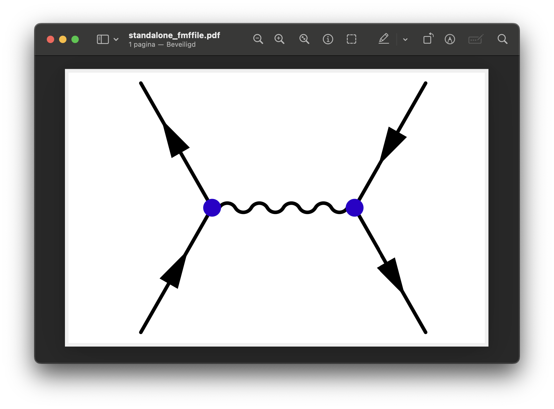
Compiling standalone diagrams
Standalone compilation is useful to create a single .tex file that creates a single PDF that you can then import into other projects as an image. If you include this standalone PDF in LaTeX documents with \includegraphics, it will save some compilation time, keeps the code clean, and you can easily reuse the same compiled image in other projects.
A simple example using the standalone document class and the feynmp-auto package for easy compilation:
\documentclass[11pt,border=4pt]{standalone}
\usepackage{feynmp-auto}
\begin{document}
\begin{fmffile}{feyngraph}
  \begin{fmfgraph*}(100,70) % dimensions (WH)
    \fmfleft{i2,i1}
    \fmfright{o2,o1}
    \fmf{fermion}{i2,v1,i1}
    \fmf{boson}{v1,v2}
    \fmf{fermion}{o1,v2,o2}
    \fmfv{decor.shape=circle,decor.filled=full,decor.size=4,
          foreground=(0,,0,,0.8)}{v1,v2}
  \end{fmfgraph*}
\end{fmffile}
\end{document}
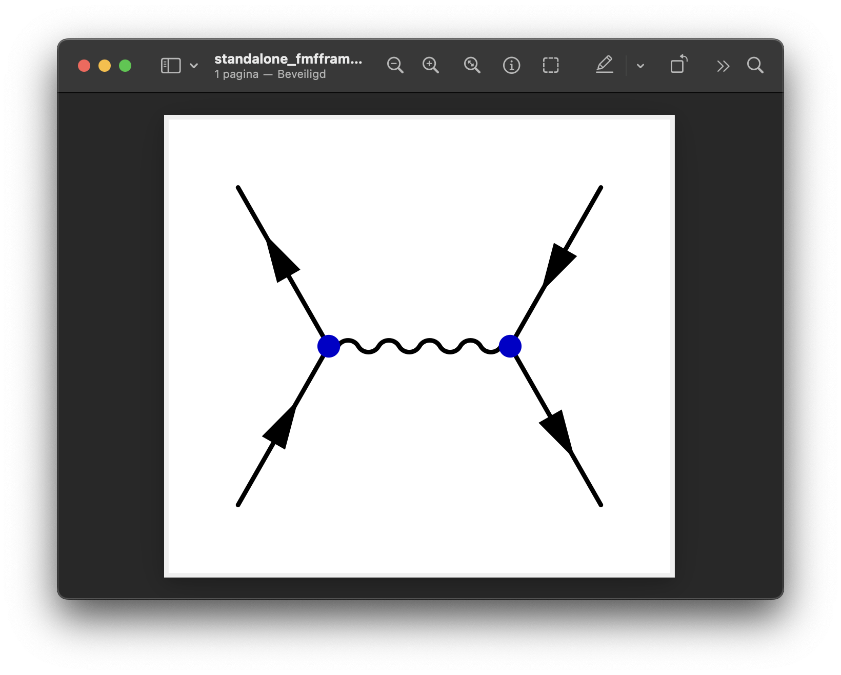
You can change the default margins by changing border=4pt in \documentclass. One can further control the whitespace around the Feynman diagram, by wrapping the fmffile or fmfgraph with \fmfframe. This command takes two pairs of floats as arguments: \fmfframe(L,T)(R,B), where L, T, R, and B are float values of the left, top, right, and bottom margin, respectively. Unfortunately, this needs to be fine-tuned sometimes, especially if you add the text labels to the external vertices.
For example:
\documentclass[11pt,border=4pt]{standalone}
\usepackage{feynmp-auto}
\begin{document}
\begin{fmffile}{feyngraph}
  \fmfframe(-5,12)(-5,12){ % padding (L,T)(R,B)
  \begin{fmfgraph*}(100,70) % dimensions (WH)
    \fmfleft{i2,i1}
    \fmfright{o2,o1}
    \fmf{fermion}{i2,v1,i1}
    \fmf{boson}{v1,v2}
    \fmf{fermion}{o1,v2,o2}
    \fmfv{decor.shape=circle,decor.filled=full,decor.size=4,
          foreground=(0,,0,,0.8)}{v1,v2}
  \end{fmfgraph*}
  } % close \fmfframe
\end{fmffile}
\end{document}
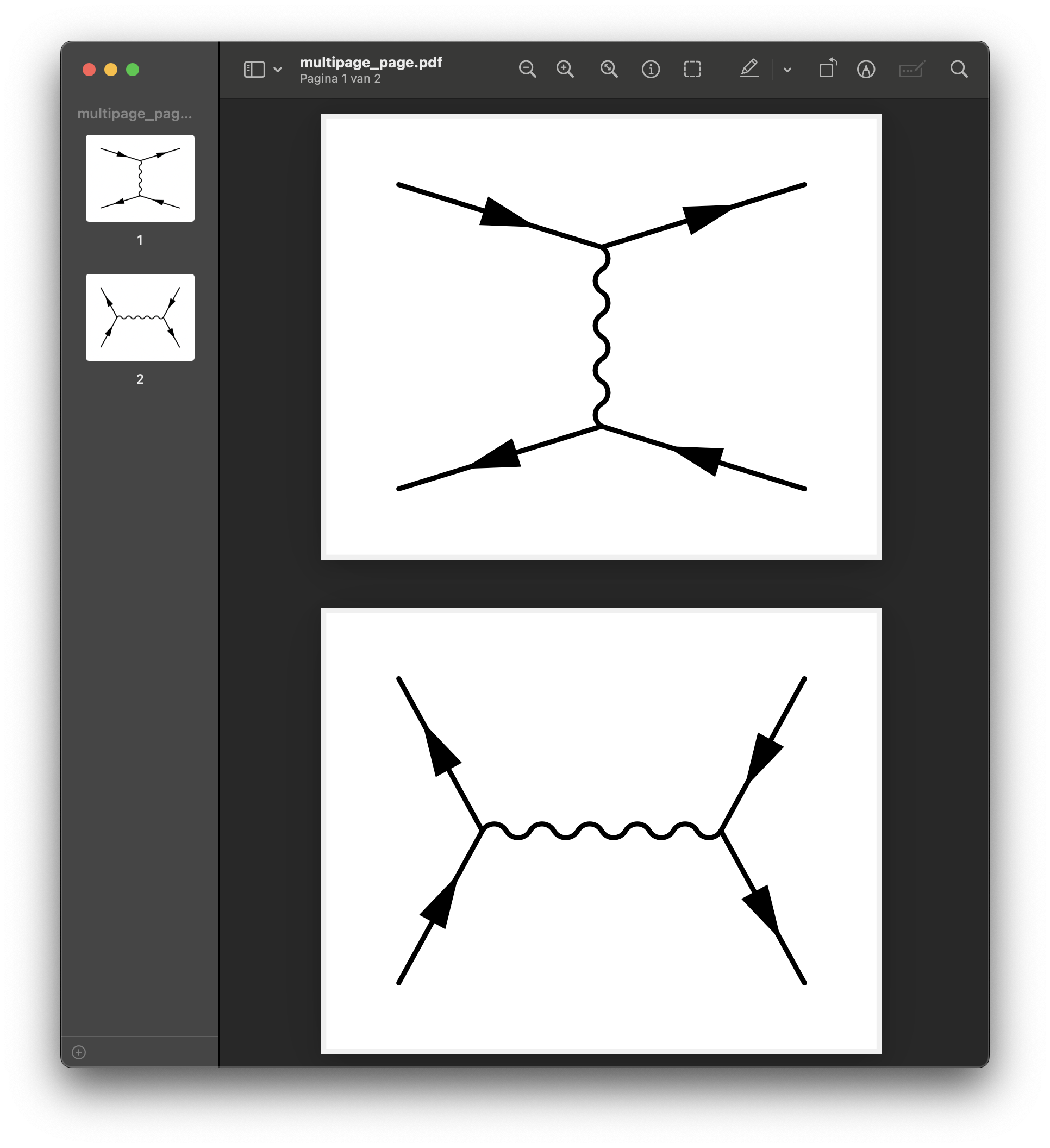
Compiling multiple standalone diagrams (multipage)
If you add more than one fmffile or tikzpicture environment in a standalone LaTeX document, the compiled PDF will contain multiple diagrams. This can be handy if you like everything in one place, where it is easier to maintain (all the code in one LaTeX file, all the diagrams in one PDF), create variations, and use some common settings like line or color style. For more information on that, see the tutorial for using color in feynmp.
To import a particular page from a multipage PDF into a LaTeX, you can use something like
\includegraphics[width=0.25\textwidth,page=2]{fig/myfeyn.pdf}
To actually produce a multipage PDF document with each Feynman diagram on a separate page, you need to explicitly wrap the fmffile in an page environment as follows:
\documentclass[11pt,border=4pt,multi=page,crop]{standalone}
\usepackage{feynmp-auto}
\begin{document}

% DIAGRAM 1
\begin{page}% to create standalone page
\begin{fmffile}{feynmp-diagram1}
  \fmfframe(-6,10)(-6,10){ % padding (L,T)(R,B)
  \begin{fmfgraph*}(100,60) % dimensions (WH)
    \fmfleft{i2,i1}
    \fmfright{o2,o1}
    \fmf{fermion}{i1,v1,o1}
    \fmf{boson,tension=0.7}{v1,v2} % t-channel
    \fmf{fermion}{o2,v2,i2}
  \end{fmfgraph*}
  }% close \fmfframe
\end{fmffile}
\end{page}

% DIAGRAM 2
\begin{page}% to create standalone page
\begin{fmffile}{feynmp-diagram2}
  \fmfframe(-6,10)(-6,10){ % padding (L,T)(R,B)
  \begin{fmfgraph*}(100,60) % dimensions (WH)
    \fmfleft{i2,i1}
    \fmfright{o2,o1}
    \fmf{fermion}{i2,v1,i1}
    \fmf{boson,tension=0.7}{v1,v2} % s-channel
    \fmf{fermion}{o1,v2,o2}
  \end{fmfgraph*}
  }% close \fmfframe
\end{fmffile}
\end{page}

\end{document}
Once you start adding more common settings, this can get a bit cumbersome to maintain. It might be useful to define a custom environment. In the following, a new environment called fmfpicture is defined with \NewEnviron. It takes three arguments: The first two set the padding with \fmfframe, and the third one passes a name to fmffile for the external MetaPost files.
\documentclass[11pt,border=4pt,multi=page,crop]{standalone}
\usepackage{feynmp-auto}

% DEFINE fmfpicture ENVIRONMENT
\usepackage{environ} % for \NewEnviron
\NewEnviron{fmfpicture}[3]{%
  \begin{page}% to create standalone page
    \fmfframe(#1)(#2){% padding (L,T)(R,B)
    \begin{fmffile}{feynmp-#3}% auxiliary files (use unique name!)
      \BODY % main code
    \end{fmffile}
    }% close \fmfframe
  \end{page}
}

\begin{document}

% DIAGRAM 1
\begin{fmfpicture}{-2,10}{-2,10}{diagram1} % padding (LTRB)
  \begin{fmfgraph*}(100,60) % dimensions (WH)
    % external vertices
    \fmfleft{i2,i1}
    \fmfright{o2,o1}
    % main
    \fmf{fermion}{i1,v1,o1}
    \fmf{boson,tension=0.7}{v1,v2} % t-channel
    \fmf{fermion}{o2,v2,i2}
  \end{fmfgraph*}
\end{fmfpicture}

% DIAGRAM 2
\begin{fmfpicture}{-2,10}{-2,10}{diagram2} % padding (LTRB)
  \begin{fmfgraph*}(100,60) % dimensions (WH)
    % external vertices
    \fmfleft{i2,i1}
    \fmfright{o2,o1}
    % main
    \fmf{fermion}{i2,v1,i1}
    \fmf{boson,tension=0.7}{v1,v2} % s-channel
    \fmf{fermion}{o1,v2,o2}
  \end{fmfgraph*}
\end{fmfpicture}

% DIAGRAM 3
\begin{fmfpicture}{-2,10}{-2,10}{diagram3} % padding (LTRB)
  \begin{fmfgraph*}(100,60) % dimensions (WH)
    % external vertices
    \fmfleft{i2,i1}
    \fmfright{o2,o1}
    % main
    \fmf{fermion}{i1,v1}
    \fmf{fermion}{v2,i2}
    \fmf{fermion,tension=0.7}{v1,v2} % t-channel
    \fmf{boson}{v1,o1}
    \fmf{boson}{o2,v2}
  \end{fmfgraph*}
\end{fmfpicture}

\end{document}
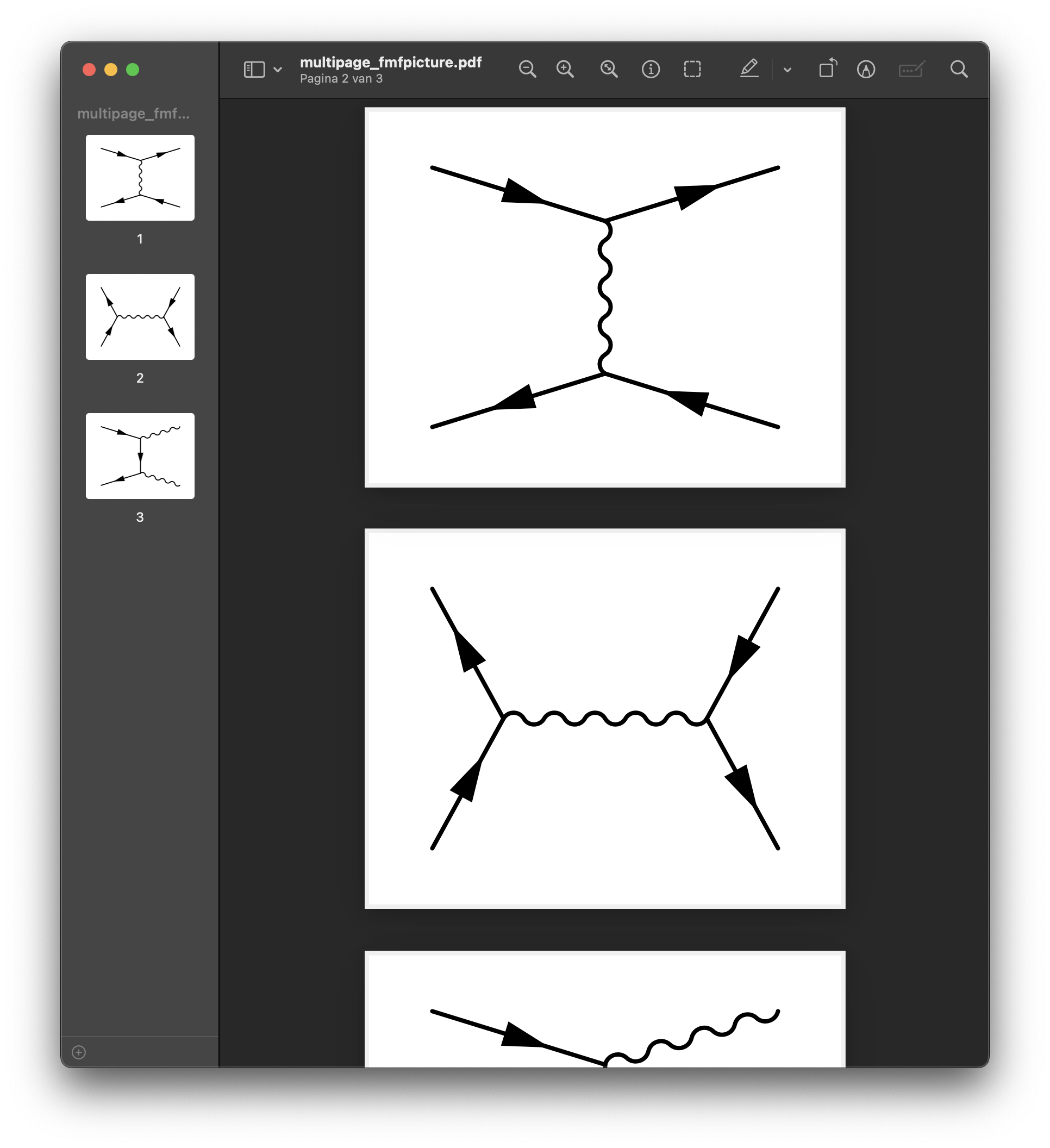
Note the placement of % behind some LaTeX code without any white space in-between. This is to prevent LaTeX from adding spurious spaces that increase the whitespace on the left and right of the figures.
Compiling diagrams as figures to a text (on-the-fly)
You can add the feynmp code directly to your LaTeX document so it is compiled together with your text. Note however that for large documents with many figures this can increase the compilation time. It might be preferable to produce the figures standalone as PDF images that are included (see previous section).
\documentclass[a4paper,12pt]{article}
\usepackage[margin=2.4cm]{geometry} % margins
\usepackage{amsmath}
\usepackage{graphicx}
\usepackage{feynmp-auto}
\begin{document}
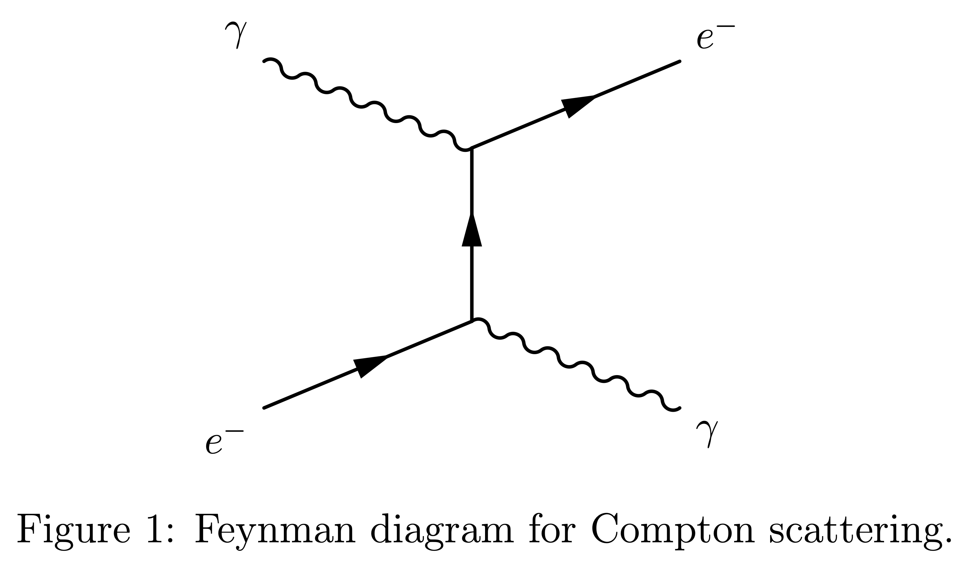
This is a test file for Feynman diagrams. You may need to compile twice: first time to compile and save the Feynman diagrams, second time to include them in the typeset PDF file.
\begin{figure}[h]
\vspace{10mm}
\centering
\begin{fmffile}{feynman-compton}
\begin{fmfgraph*}(150,100)
\fmfleft{i1,i2}
\fmfright{o1,o2}
\fmflabel{$\gamma$}{i2}
\fmflabel{$e^-$}{i1}
\fmflabel{$\gamma$}{o1}
\fmflabel{$e^-$}{o2}
\fmf{photon}{i2,v2}
\fmf{fermion}{i1,v1,v2,o2}
\fmf{photon}{v1,o1}
\end{fmfgraph*}
\end{fmffile}
\vspace{5mm}
\caption{Feynman diagram for Compton scattering} \label{compton}
\end{figure}
\end{document}
Compiling inside equations
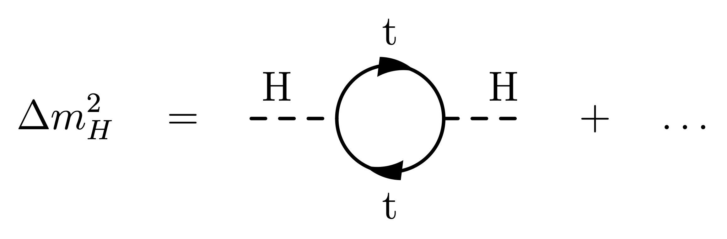
Feynman diagrams represent mathematical expressions that describe interactions of particles. It is possible to insert Feynman diagrams with feynmp in LaTeX with something like the following.
\documentclass[a4paper,12pt]{article}
\usepackage{feynmp-auto}
\begin{document}
An equation with a Feynman diagram:
\begin{equation}\label{eq:higgs_mass}
  \begin{fmffile}{higgs_mass}
    \Delta m_H^2
    \quad = \quad \parbox{80pt}{
    \begin{fmfgraph*}(80,60)
      \fmfleft{i}
      \fmfright{o}
      \fmfv{label=H,l.a=60}{i}
      \fmfv{label=H,l.a=120}{o}
      \fmf{dashes,tension=1}{i,v1}
      \fmf{dashes,tension=1}{v2,o}
      \fmf{fermion,left,tension=0.4,label=t}{v1,v2,v1}
    \end{fmfgraph*}}
    \quad + \quad\ldots
  \end{fmffile}
\end{equation}
\end{document}
A full example, shown how the finetuning problem of the Higgs mass can be solved with loops containing new SUSY particles:
The code below shows how you can achieve this:
% !TEX program = pdflatexmk
% !TEX parameter = -shell-escape
% Author: Izaak Neutelings (July 2017)
\documentclass[a4paper,12pt]{article}
\usepackage[margin=2.4cm]{geometry} % margins
\usepackage{amsmath}
\usepackage{graphicx}
\usepackage{feynmp-auto}
\begin{document}
\section{Typesetting equations with Feynman diagrams}
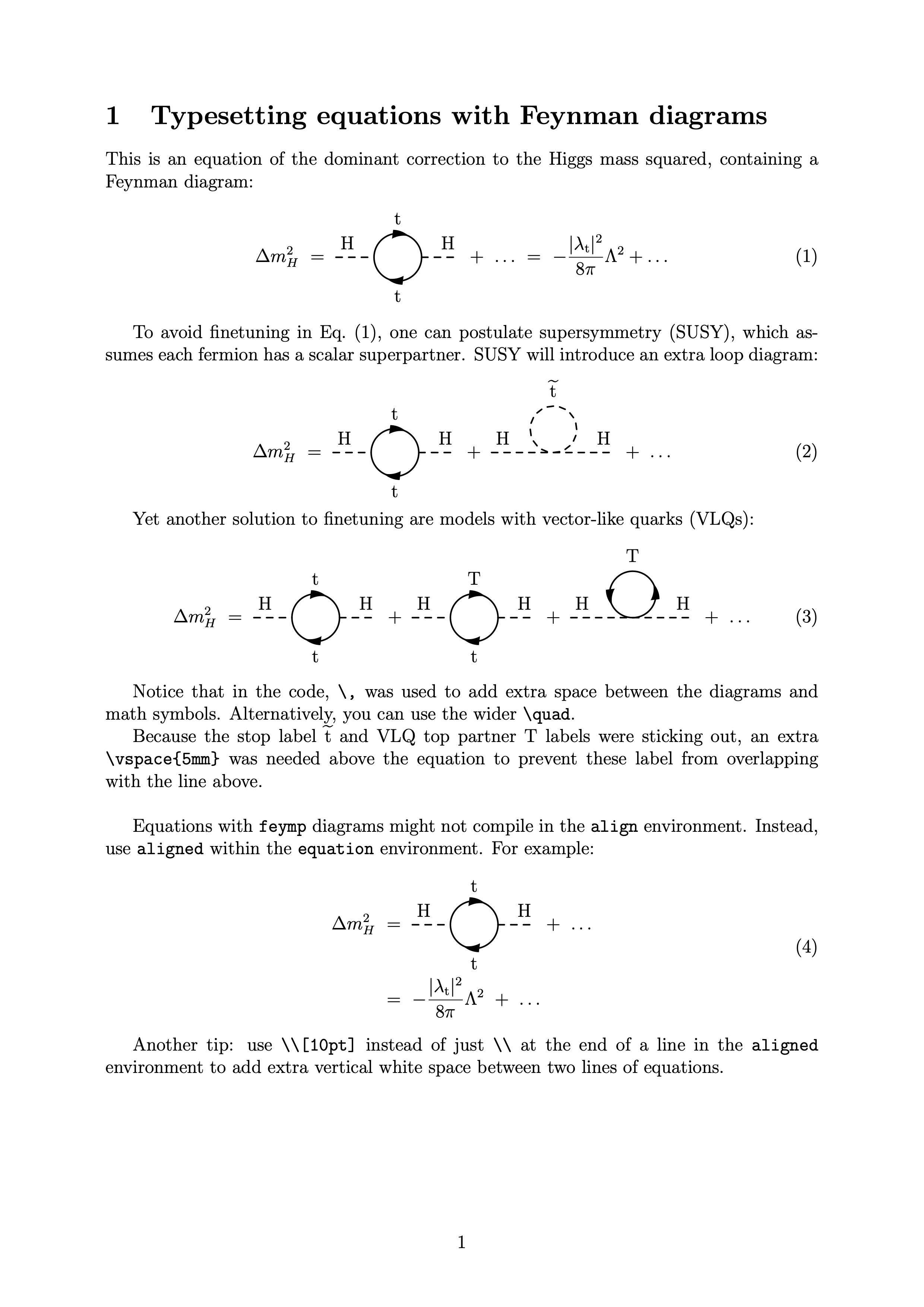
This is an equation of the dominant correction to the Higgs mass squared, containing a Feynman diagram:
\begin{equation}\label{eq:hierarchy_problem}
\begin{fmffile}{higgs_mass_correction}
\Delta m_H^2
\,\, = \,\,\parbox{80pt}{
\begin{fmfgraph*}(80,60)
\fmfleft{i}
\fmfright{o}
\fmfv{label=H,l.a=60}{i}
\fmfv{label=H,l.a=120}{o}
\fmf{dashes,tension=1}{i,v1} % ,label=H,label.side=left
\fmf{dashes,tension=1}{v2,o}
\fmf{fermion,left,tension=0.4,label=t}{v1,v2,v1}
\end{fmfgraph*}}
\,\, + \,\,\ldots
\,\, = \,\, -\frac{|\lambda_\mathrm{t}|^2}{8\pi}\Lambda^2 + \ldots
\end{fmffile}
\end{equation}
% SUSY
To avoid finetuning in Eq.~\eqref{eq:hierarchy_problem}, one can postulate supersymmetry (SUSY), which assumes each fermion has a scalar superpartner. SUSY will introduce an extra loop diagram: \vspace{5mm}
\begin{equation}\label{eq:hierarchy_problem_SUSY}
\begin{fmffile}{higgs_mass_correction_SUSY}
\Delta m_H^2
\,\, = \,\,\parbox{80pt}{
\begin{fmfgraph*}(80,60)
\fmfleft{i}
\fmfright{o}
\fmfv{label=H,l.a=60}{i}
\fmfv{label=H,l.a=120}{o}
\fmf{dashes,tension=1}{i,v1}
\fmf{dashes,tension=1}{v2,o}
\fmf{fermion,left,tension=0.4,label=t}{v1,v2,v1}
\end{fmfgraph*}}
\,\, + \,\,\parbox{80pt}{
\begin{fmfgraph*}(80,60)
\fmfleft{i}
\fmfright{o}
\fmftop{m}
\fmfv{label=H,l.a=60}{i}
\fmfv{label=H,l.a=120}{o}
\fmflabel{$\widetilde{\mathrm{t}}$}{m}
\fmf{dashes,tension=1}{i,v1}
\fmf{dashes,tension=1}{v1,o}
\fmf{dashes,right,tension=0}{v1,m,v1}
\end{fmfgraph*}}
\,\, + \,\,\ldots
\end{fmffile}
\end{equation}
% VLQ
Yet another solution to finetuning are models with vector-like quarks (VLQs): \vspace{5mm}
\begin{equation}\label{eq:hierarchy_problem_VLQ}
\begin{fmffile}{higgs_mass_correction_VLQ}
\Delta m_H^2
\,\, = \,\,\parbox{80pt}{
\begin{fmfgraph*}(80,60)
\fmfleft{i}
\fmfright{o}
\fmfv{label=H,l.a=60}{i}
\fmfv{label=H,l.a=120}{o}
\fmf{dashes,tension=1}{i,v1}
\fmf{dashes,tension=1}{v2,o}
\fmf{fermion,left,tension=0.4,label=t}{v1,v2,v1}
\end{fmfgraph*}}
\,\, + \,\,\parbox{80pt}{
\begin{fmfgraph*}(80,60)
\fmfleft{i}
\fmfright{o}
\fmfv{label=H,l.a=60}{i}
\fmfv{label=H,l.a=120}{o}
\fmf{dashes,tension=1}{i,v1}
\fmf{dashes,tension=1}{v2,o}
\fmf{fermion,left,tension=0.4,label=t}{v2,v1}
\fmf{fermion,left,tension=0.4,label=T}{v1,v2}
\end{fmfgraph*}}
\,\, + \,\,\parbox{80pt}{
\begin{fmfgraph*}(80,60)
\fmfleft{i}
\fmfright{o}
\fmftop{m}
\fmfv{label=H,l.a=60}{i}
\fmfv{label=H,l.a=120}{o}
\fmflabel{T}{m}
\fmf{dashes,tension=1}{i,v1}
\fmf{dashes,tension=1}{v1,o}
\fmf{fermion,right,tension=0}{v1,m,v1}
\end{fmfgraph*}}
\,\, + \,\,\ldots
\end{fmffile}
\end{equation}
Notice that in the code, \verb|\,| was used to add extra space between the diagrams and math symbols. Alternatively, you can use the wider \verb|\quad|.
Because the stop label $\widetilde{\mathrm{t}}$ and VLQ top partner T labels were sticking out, an extra \verb|\vspace{5mm}| was needed above the equation to prevent these label from overlapping with the line above.\\
Equations with \verb|feymp| diagrams might not compile in the \verb|align| environment. Instead, use \verb|aligned| within the \verb|equation| environment. For example:
\begin{equation}
\begin{aligned}
\Delta m_H^2 \,\, &=
\begin{fmffile}{higgs_mass_correction}
\,\,\parbox{80pt}{
\begin{fmfgraph*}(80,60)
\fmfleft{i}
\fmfright{o}
\fmfv{label=H,l.a=60}{i}
\fmfv{label=H,l.a=120}{o}
\fmf{dashes,tension=1}{i,v1}
\fmf{dashes,tension=1}{v2,o}
\fmf{fermion,left,tension=0.4,label=t}{v1,v2,v1}
\end{fmfgraph*}}
\,\, + \,\,\ldots
\end{fmffile}\\ %[10pt] % to add extra vertical white space between the line
&= \,\, -\frac{|\lambda_\mathrm{t}|^2}{8\pi}\Lambda^2 \,\, + \,\,\ldots
\end{aligned}
\end{equation}
Another tip: use \verb|\\[10pt]| instead of just \verb|\\| at the end of a line in the \verb|aligned| environment to add extra vertical white space between two lines of equations.
\end{document}
Compiling standalone with LaTeXiT (macOS)
LaTeXiT by Pierre Chatelier is a very nice macOS application that typesets LaTeX code as standalone images (JPG, PNG, PDF, …). This is extremely useful for preparing high-quality equations in PowerPoint presentations. LaTeXiT can create standalone images Feynman diagram with the feynmp package. It requires some special configuration though, which are explained below. These steps are based on the instructions by Taku Yamanaka on this page.
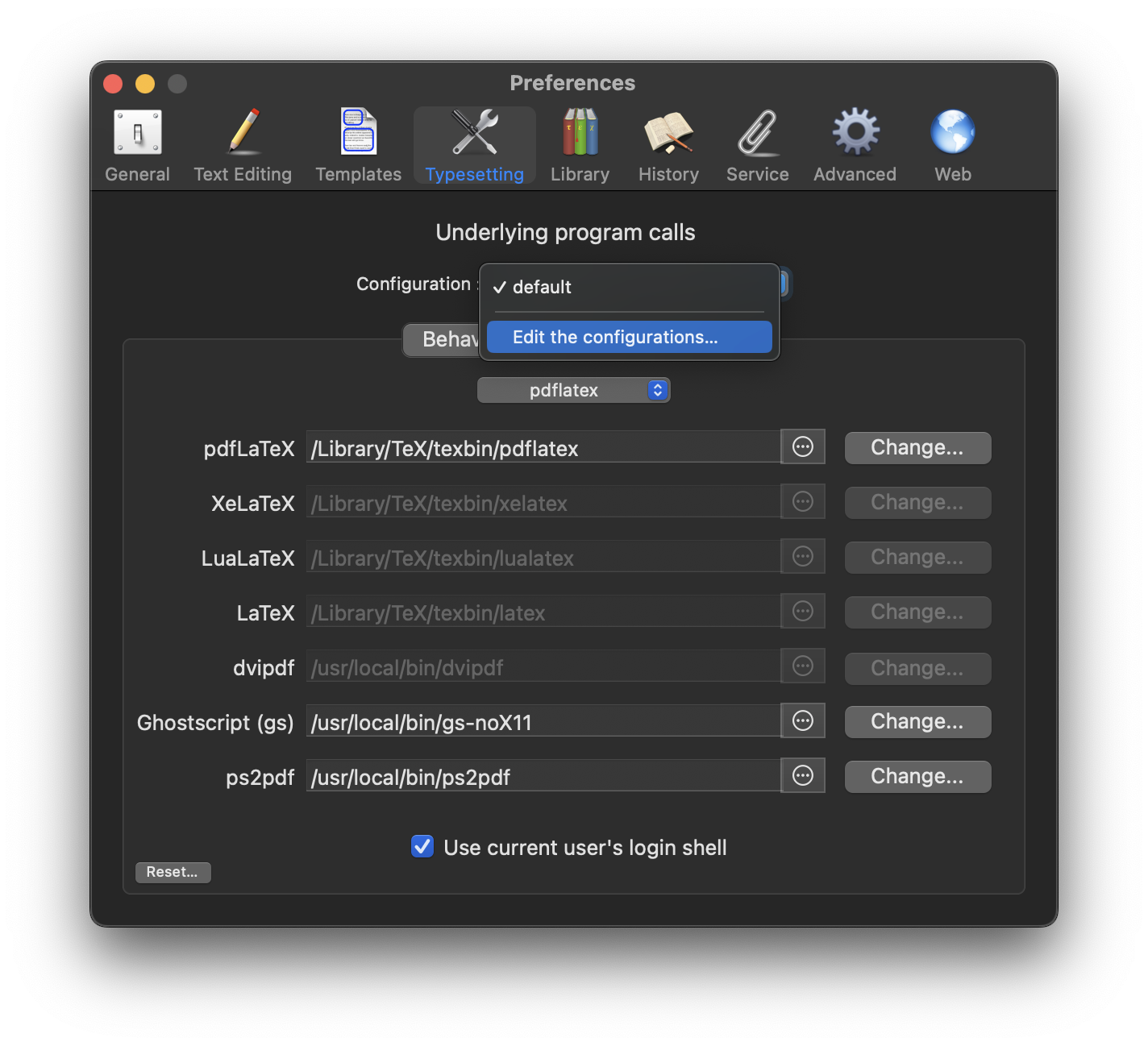
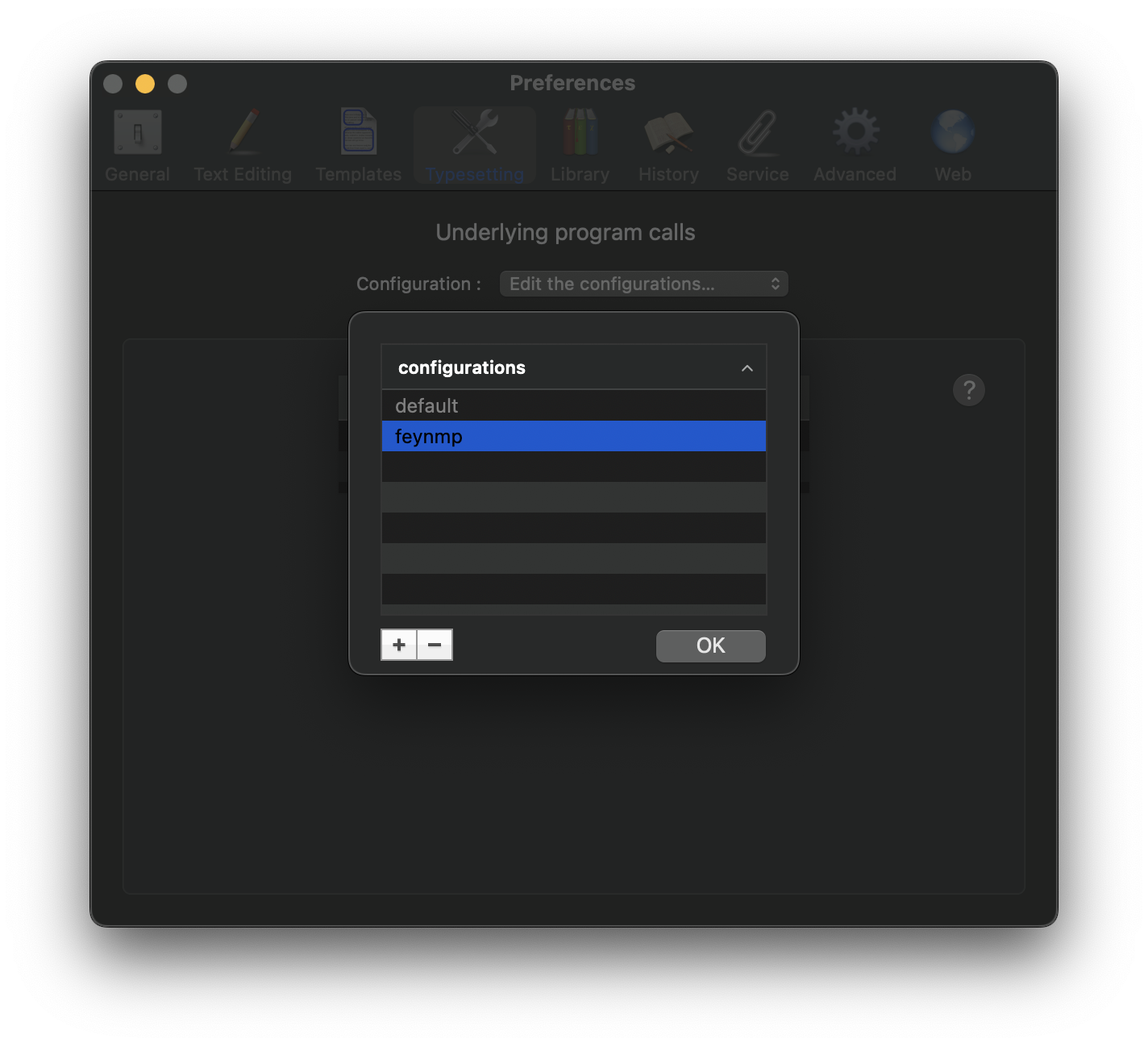
Step 1. Open the LaTeXiT preference panel from the menu bar on the top via “LaTeXiT” > “Settings…”, or use the shortcut ⌘, and go to the “Typesetting” tab, where you click “Edit the configurations…” in the drop-down menu:
Step 2. In the panel, add a new configuration by clicking the “+” button on the bottom left, and give it some name like “feynmp” and click “OK”:
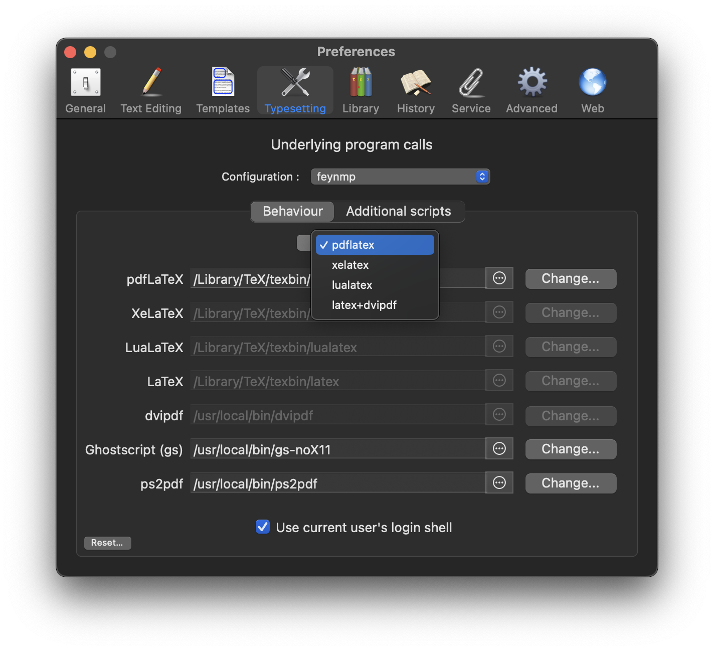
Step 3. While the new configuration is selected, make sure the compiler correctly select. Either “pdflatex” or “latex+dvipdf” should work.
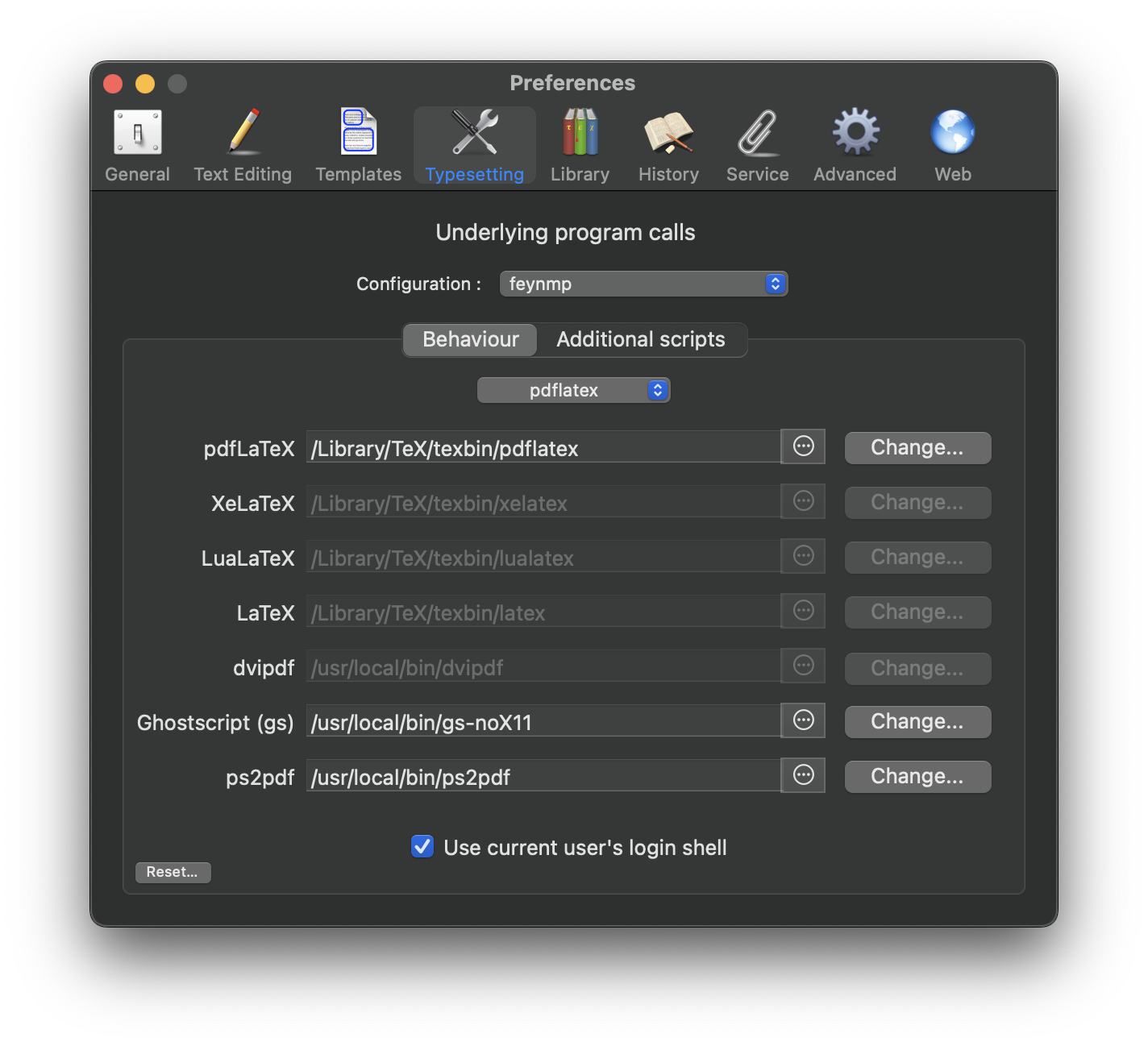
Step 4. The default paths should be fine, but it may depend on your system and how LaTeX was installed. The paths in the screenshot below are for macOS Ventura 13.7 with LaTeX installed by the MacTex 2022 package.
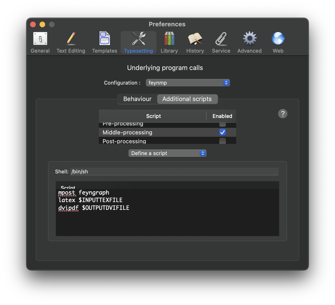
Step 5. Now we setup a special script that compiles the intermediate MetaPost files. Go to the “Additional scripts” subtab and enable the “Middle-processing” script by ticking off the checkbox next to it. While this row is selected, add the following three lines to the field to the “Define a script” option:
  mpost feyngraph

  latex $INPUTTEXFILE

  dvipdf $OUTPUTDVIFILE
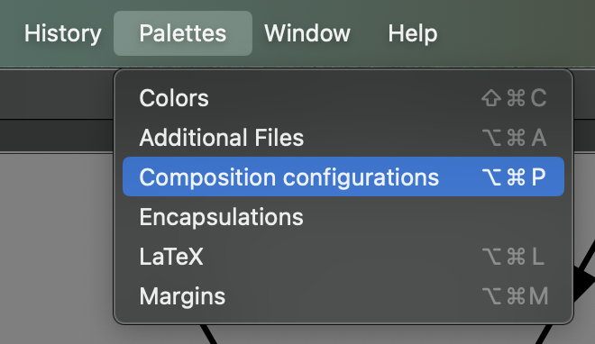
Step 6. Now open a new LaTeX editor window under “File” > “New” or with the shortcut ⌘N. Then make sure you have the new configuration set. Go to “Palettes” > “Compositions configurations” or with the shortcut ⌥⌘P. In the “Compositions configurations” panel select the “feynmp” configuration (or whatever you called it).
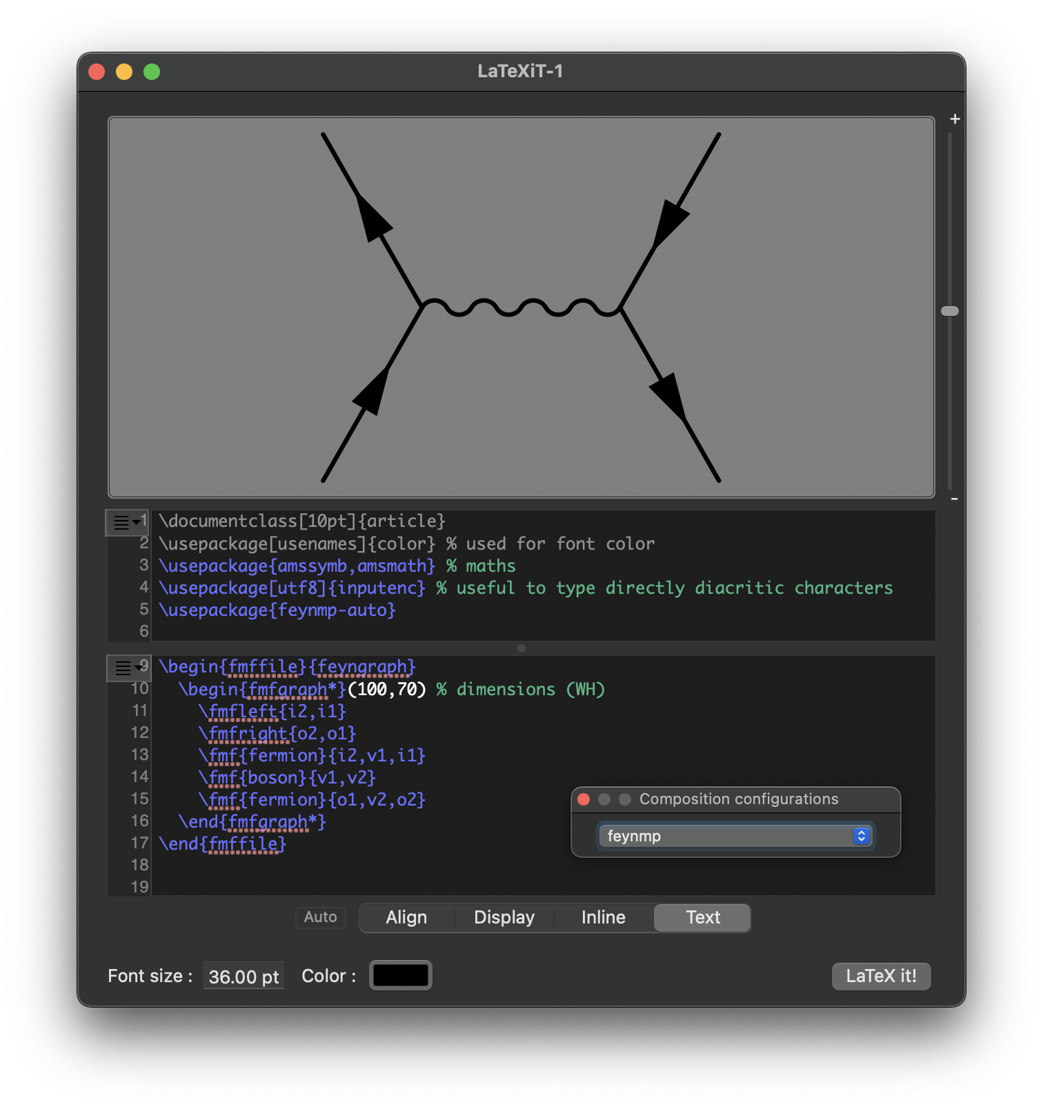
Step 7. Now we can go ahead and compile Feynman diagrams! Add \usepackage{feynmp-auto} in the top field for the preamble, and add the main code in the bottom field while having the “Text” option selected, as shown below:
  \begin{fmffile}{feyngraph}

    \begin{fmfgraph*}(100,70) % dimensions (WH)

      \fmfleft{i2,i1}

      \fmfright{o2,o1}

      \fmf{fermion}{i2,v1,i1}

      \fmf{boson}{v1,v2}

      \fmf{fermion}{o1,v2,o2}

    \end{fmfgraph*}

  \end{fmffile}
Now you’re good to go! You can drag the diagram from the display to the desktop or some folder as a PNG, PDF, JPG, … image file.
As a final tip: LaTeXiT has a very nice and useful feature that the source code is encoded in the metadata of the image files it creates. This allows you to drag back the image file to a LaTeXiT window so you can view and edit the code again.
Compiling standalone with TeXShop
Many LaTeX editors recognize “TeX magic comments” that are included on top of the document to pick the right compilation method and options. These lines start with % !TEX.
If you use the TeXShop editor on macOS, you can include the following at the top of your document:
  % !TEX program = pdflatexmk

  % !TEX parameter = -shell-escape
This will automatically compile the diagrams with pdflatex -shell-escape. Note that pdflatexmk is a default “engine” script for TeXShop that can be found in ~/Library/TeXShop/Engines/.
Compiling standalone with VSCode
There are many people who use the Visual Studio Code (VSCode) editor for programming, including to write and compile their LaTeX documents locally with the popular LaTeX Workshop extension by James Yu. Here are some tips to configure LaTeX Workshop in VSCode.
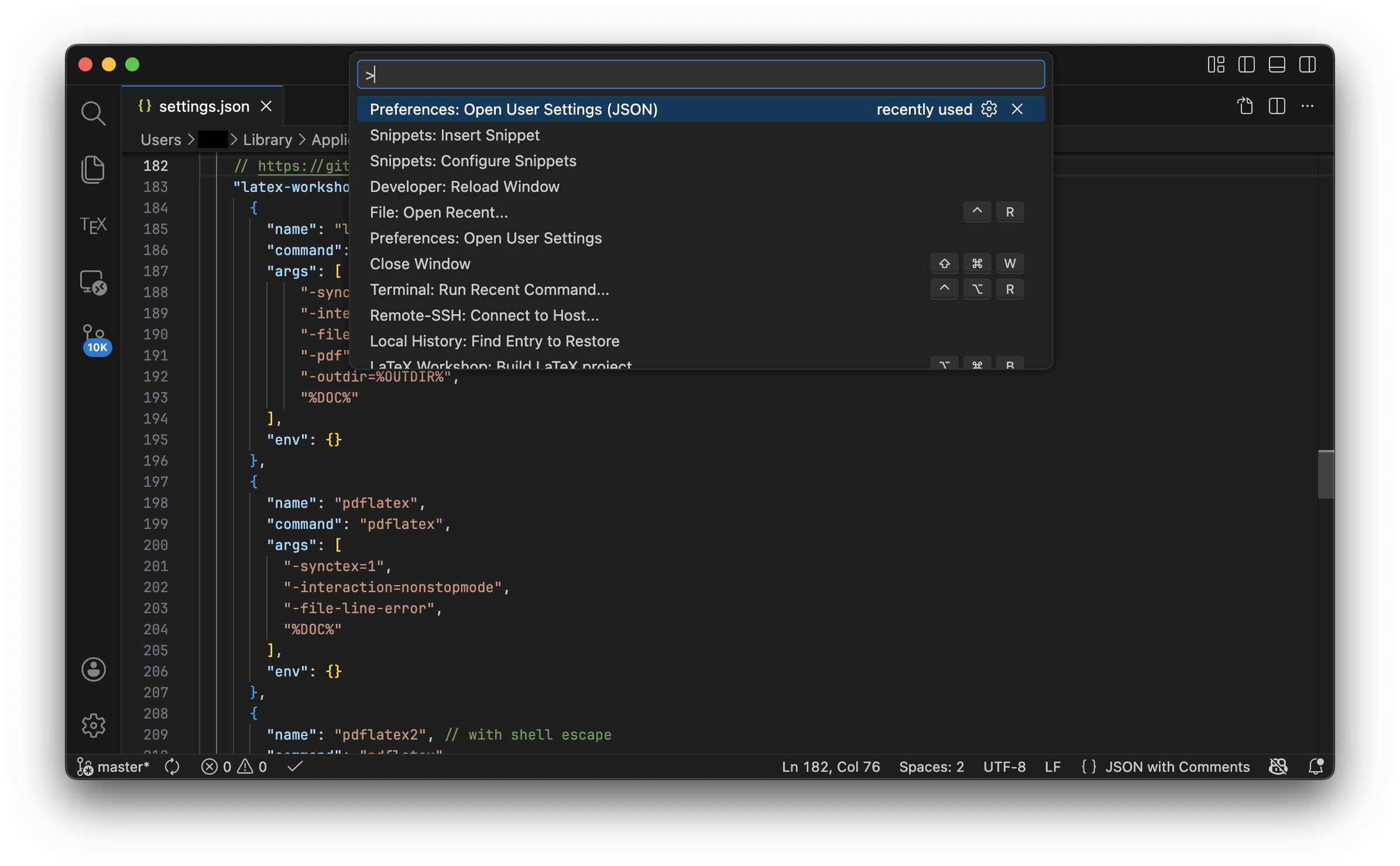
First, open your main user settings JSON file called settings.json. There are several ways, as outlined in the official documentation. You can first open the Command Palette from the “View” drop-down menu, or with the short key ⇧⌘P for macOS, or Ctrl+Shift+P for Windows and Linux. Choose “Preferences: Open User Settings (JSON)”. You can type this in the Command Palette if needed.
Then in settings.json, you can add something like the following lines to configure LaTeX Workshop:
    // ...

    "latex-workshop.latex.tools": [

      {

        "name": "latexmk",

        "command": "latexmk",

        "args": [

            "-synctex=1",

            "-interaction=nonstopmode",

            "-file-line-error",

            "-pdf",

            "-outdir=%OUTDIR%",

            "%DOC%"

        ],

        "env": {}

      },

      {

        "name": "pdflatex",

        "command": "pdflatex",

        "args": [

          "-synctex=1",

          "-interaction=nonstopmode",

          "-file-line-error",

          "%DOC%"

        ],

        "env": {}

      },

      {

        "name": "pdflatex2", // with shell escape

        "command": "pdflatex",

        "args": [

          "-shell-escape",

          "-synctex=1",

          "-interaction=nonstopmode",

          "-file-line-error",

          "%DOC%"

        ],

        "env": {}

      },

      {

        "name": "bibtex",

        "command": "bibtex",

        "args": [

          "%DOCFILE%"

        ],

        "env": {}

      }

    ],

    "latex-workshop.latex.recipes": [

      {

        "name": "latexmk",

        "tools": ["latexmk"]

      },

      {

        "name": "pdflatex",

        "tools": ["pdflatex"]

      },

      { // twice with shell escape, e.g. for feynmp

        "name": "pdflatex2",

        "tools": ["pdflatex2","pdflatex2"]

      },

      {

        "name": "pdflatex+bibtex",

        "tools": ["pdflatex","bibtex","pdflatex","pdflatex"]

      }

    ],

    "latex-workshop.latex.recipe.default": "pdflatex",

    "latex-workshop.latex.autoBuild.run": "never",

    "latex-workshop.latex.clean.method": "glob", // allow * wildcards

    "latex-workshop.latex.clean.fileTypes": [

      "%DOCFILE%.bbl", "%DOCFILE%.blg", "%DOCFILE%.idx", "%DOCFILE%.ind",

      "%DOCFILE%.lof", "%DOCFILE%.lot", "%DOCFILE%.toc",

      "%DOCFILE%.acn", "%DOCFILE%.acr", "%DOCFILE%.alg",

      "%DOCFILE%.glg", "%DOCFILE%.glo", "%DOCFILE%.gls", "%DOCFILE%.fls",

      "%DOCFILE%.aux", "%DOCFILE%.log", "%DOCFILE%.out",

      "%DOCFILE%.synctex.gz", "%DOCFILE%.synctex(busy)", "%DOCFILE%.synctex.gz(busy)",

      "%DOCFILE%.fdb_latexmk", "%DOCFILE%.snm", "%DOCFILE%.nav", "%DOCFILE%.vrb",

      "feyn*.1", "feyn*.mp", "feyn*.log" // feynm MetaPost files

    ],

    // ...
The lines relevant specifically for compiling feynmp diagrams are those related to setup the pdflatex2 script (“tool”) and recipe of the same name. This recipe simply compiles the LaTeX document twice with pdflatex and the -shell-escape flag. More information can be found the official LaTeX Workshop documentation.
To compile, first make sure you have the LaTeX document selected and then go to the LaTeX Workshop tab in the sidebar, find “Recipe: pdflatex2” under “Build LaTeX project”. It should immediately compile the PDF, which you can view by clicking the “View LaTeX PDF”, or the icon with the magnifying glass symbol on the top right.
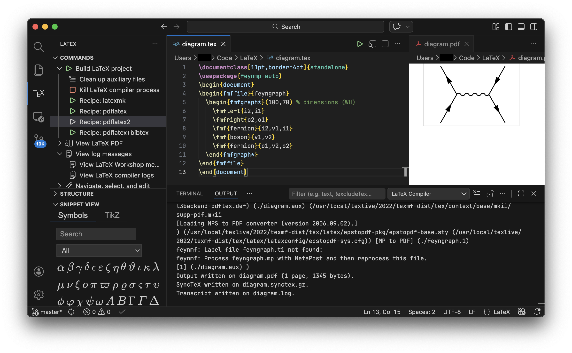
If you have problems, look at the LaTeX Workshop logs by clicking “View log messages”, or “View LaTeX compiler logs” for issues related to the LaTeX code in your document. Sometimes it’s worth starting from scratch by deleting all auxiliary files by clicking “Clean up auxiliary files”.
As a final tip, you can configure this cleaning method to also delete the auxiliary MetaPost files by adding something like "feyn*.1", "feyn*.mp", "feyn*.log" to the latex-workshop.latex.clean.fileTypes list in settings.json if your fmffile names always start with feyn, for example. However, make sure to also add "latex-workshop.latex.clean.method": "glob", to allow for glob patterns like the * wildcards.