This page is under construction. It will be based on this page.
The feynmp package is basically a nice user-friendly interface to its real engine, MetaPost.
The next level of mastering the feynmp is using “intermediate mode” with \fmfiv and \fmfi, or executing MetaPost commands directly with \fmfcmd. This gives you more control over the diagram, and allows you to construct more complicated diagrams that the usual command do not allow you to. This website contains many examples of more advanced diagrams, some of which are shown at the bottom of this page.
The content of this page:
Overview
The relation of vertex and lines versus the MetaPost pairs and paths that are accessible via intermediate mode are illustrated in the figure below from the feynFM manual:
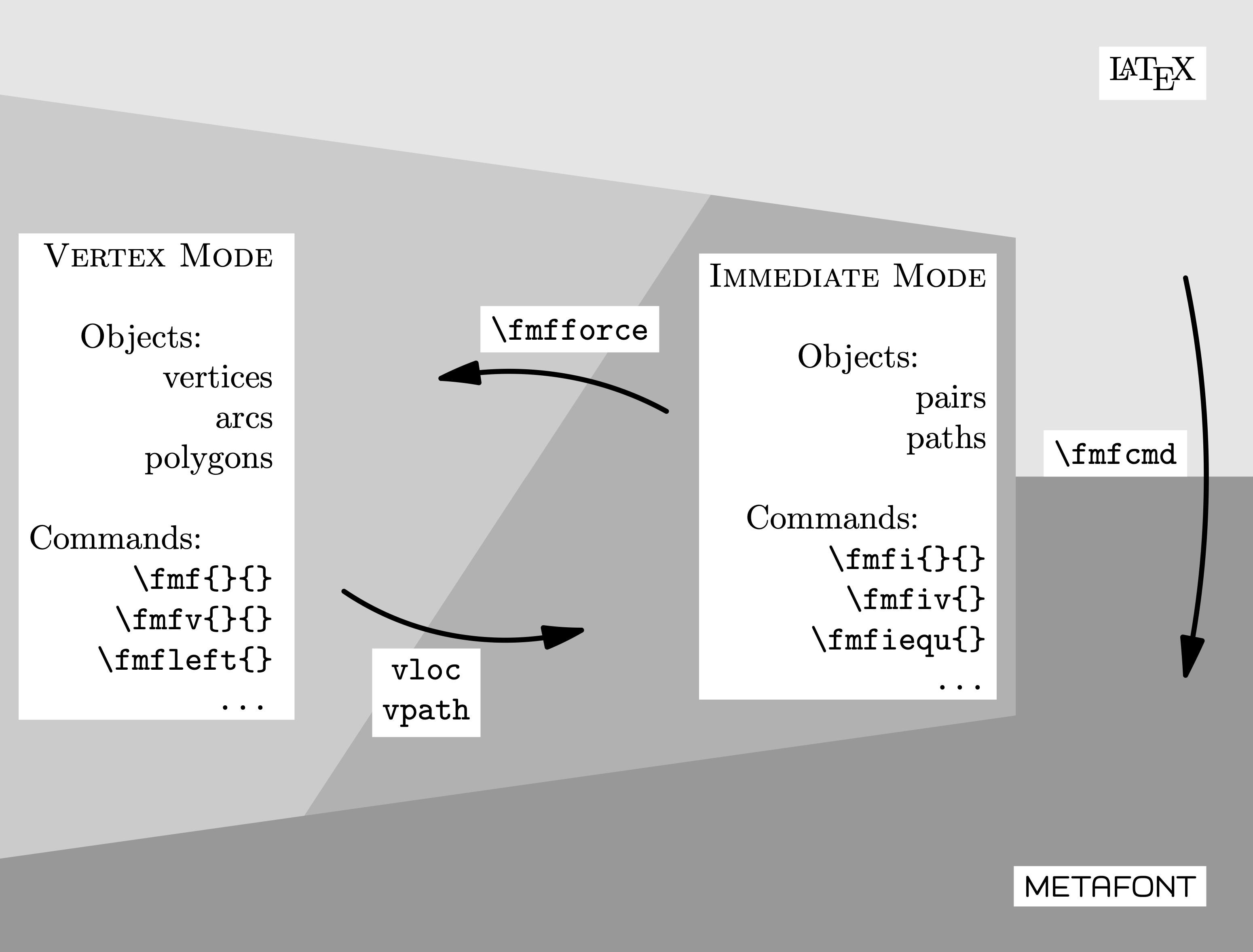
You can learn more about MetaPost in the official manual or this tutorial. The feynMF manual and this paper by the author, Thorsten Ohl contain some examples, and the author also put some advanced ones on this webpage.
Vertices: MetaPost pairs
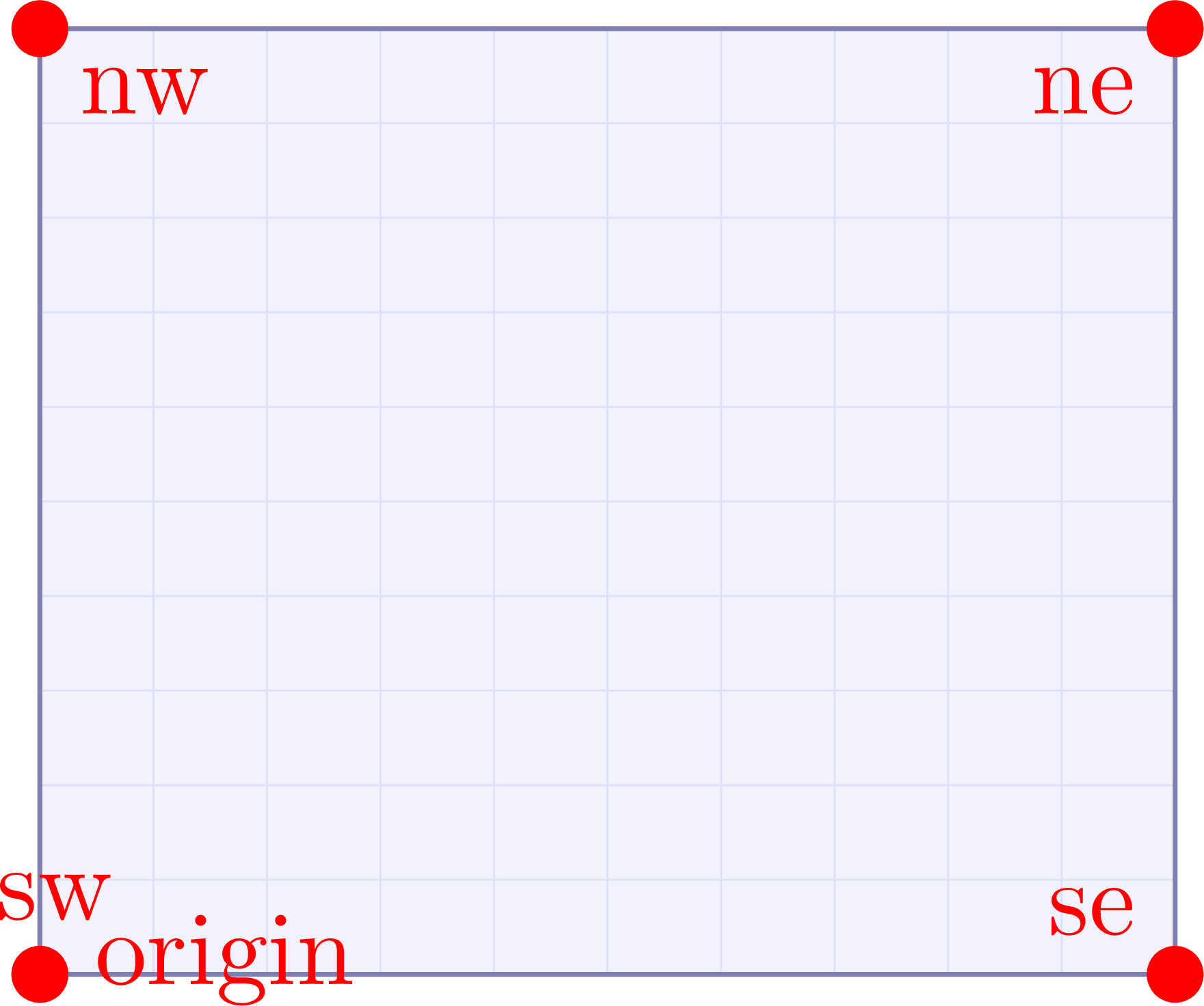
There are already some predefined points like origin and the cardinal directions ne (northeast), nw (northwest), se (southeast) and sw (southwest) for each corner.
\documentclass[11pt,border=4pt]{standalone}
\usepackage{feynmp-auto}
\begin{document}
\begin{fmffile}{feyngraph}
  \begin{fmfgraph*}(120,100) % dimensions (WH)
    % predefined points (MetaPost pairs)
    \fmfiv{d.sh=circle,d.f=1,d.si=5pt,l.a=15,l=origin}{origin}
    \fmfiv{d.sh=circle,d.f=1,d.si=5pt,l.a=-135,l=ne}{ne}
    \fmfiv{d.sh=circle,d.f=1,d.si=5pt,l.a=-45,l=nw}{nw}
    \fmfiv{d.sh=circle,d.f=1,d.si=5pt,l.a=135,l=se}{se}
    \fmfiv{d.sh=circle,d.f=1,d.si=5pt,l.a=75,l=sw}{sw}
  \end{fmfgraph*}
\end{fmffile}
\end{document}
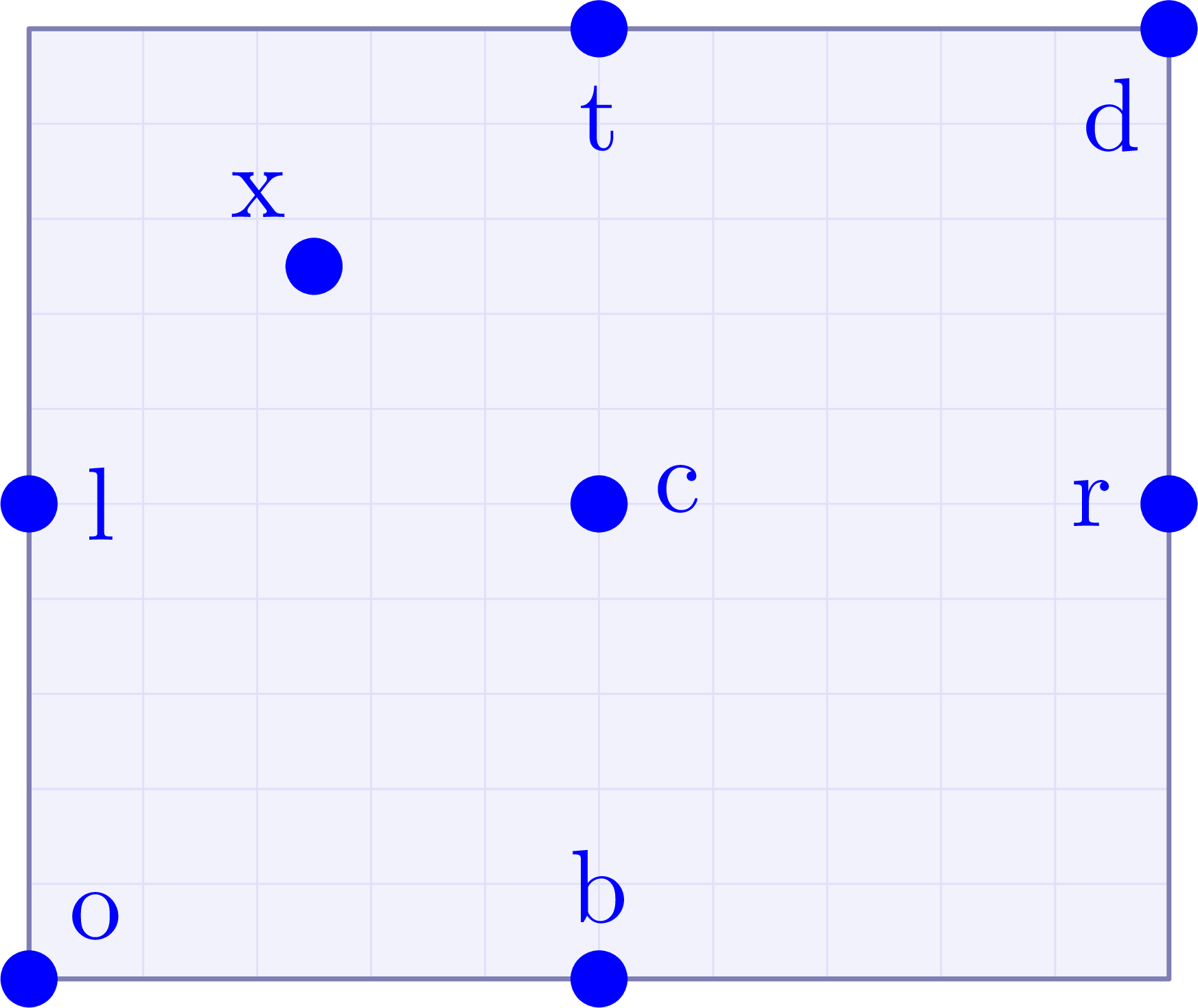
Vertices in the intermediate mode have to be first declared as MetaPost pairs with \fmfipair. After that, you can set them in several different ways. Here are some examples using explicit coordinates, scaled by the width and height via w and h, respectively:
\documentclass[11pt,border=4pt]{standalone}
\usepackage{feynmp-auto}
\begin{document}
\begin{fmffile}{feyngraph}
  \begin{fmfgraph*}(120,100) % dimensions (WH)
    % define new points with coordinates
    \fmfipair{o,c,d,l,r,t,b,x} % declare MetaPost pair
    \fmfiequ{o}{(0,0)}
    \fmfiequ{l}{(0w,0.5h)}
    \fmfiequ{c}{(0.5w,0.5h)}
    \fmfiequ{r}{(1w,0.5h)}
    \fmfiequ{d}{(1w,1h)}
    \fmfiequ{t}{(0.5w,1h)}
    \fmfiequ{b}{(0.5w,0h)}
    \fmfiequ{x}{(0.25w,0.75h)}
    % draw new coordinates with labels
    \fmfiv{d.sh=circle,d.f=1,d.si=5pt,l.a=45,l=o}{o}
    \fmfiv{d.sh=circle,d.f=1,d.si=5pt,l.a=0,l=l}{l}
    \fmfiv{d.sh=circle,d.f=1,d.si=5pt,l.a=15,l=c}{c}
    \fmfiv{d.sh=circle,d.f=1,d.si=5pt,l.a=180,l=r}{r}
    \fmfiv{d.sh=circle,d.f=1,d.si=5pt,l.a=-120,l=d}{d}
    \fmfiv{d.sh=circle,d.f=1,d.si=5pt,l.a=-90,l=t}{t}
    \fmfiv{d.sh=circle,d.f=1,d.si=5pt,l.a=90,l=b}{b}
    \fmfiv{d.sh=circle,d.f=1,d.si=5pt,l.a=120,l=x}{x}
  \end{fmfgraph*}
\end{fmffile}
\end{document}
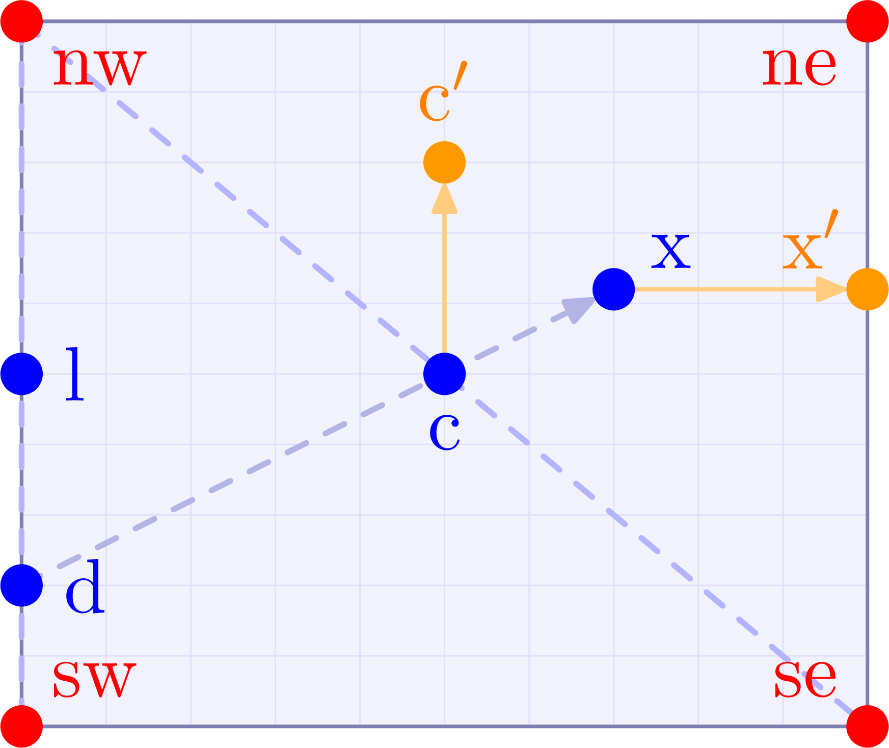
However, there are some convenient operations one can do, like vectorial adding two pairs, or setting the pair along a straight line through two other pairs, etc.
\documentclass[11pt,border=4pt]{standalone}
\usepackage{feynmp-auto}
\begin{document}
\begin{fmffile}{feyngraph}
  \begin{fmfgraph*}(120,100) % dimensions (WH)
    % predefined points (MetaPost pairs)
    \fmfiv{d.sh=circle,d.f=1,d.si=5pt,l.a=-135,l=ne}{ne}
    \fmfiv{d.sh=circle,d.f=1,d.si=5pt,l.a=-45,l=nw}{nw}
    \fmfiv{d.sh=circle,d.f=1,d.si=5pt,l.a=135,l=se}{se}
    \fmfiv{d.sh=circle,d.f=1,d.si=5pt,l.a=45,l=sw}{sw}
    % define new points with coordinates
    \fmfipair{l,c,c',d,x,x'} % declare MetaPost pairs
    \fmfiequ{l}{0.5[nw,sw]} % interpolate nw--sw
    \fmfiequ{c}{0.5[nw,se]} % interpolate nw--se
    \fmfiequ{d}{0.2[sw,nw]} % interpolate nw--nw
    \fmfiequ{x}{1.4[d,c]}   % extrapolate
    % define new point with projection
    \fmfiequ{ypart(x')}{ypart(x)} % set y coordinate of x'
    \fmfiequ{xpart(x')}{xpart(.5[ne,se])} % set y coordinate of x'
    % define new point with relative coordinate
    \fmfiequ{c'}{c+(0,.3h)} % vertical offset
    % draw new coordinates with labels
    \fmfiv{d.sh=circle,d.f=1,d.si=5pt,l.a=0,l=l}{l}
    \fmfiv{d.sh=circle,d.f=1,d.si=5pt,l.a=-90,l=c}{c}
    \fmfiv{d.sh=circle,d.f=1,d.si=5pt,l.a=0,l=d}{d}
    \fmfiv{d.sh=circle,d.f=1,d.si=5pt,l.a=30,l=x}{x}
    \fmfiv{d.sh=circle,d.f=1,d.si=5pt,l.a=140,l.d=4.6,l=x$'$}{x'}
    \fmfiv{d.sh=circle,d.f=1,d.si=5pt,l.a=90,l=c$'$}{c'}
  \end{fmfgraph*}
\end{fmffile}
\end{document}
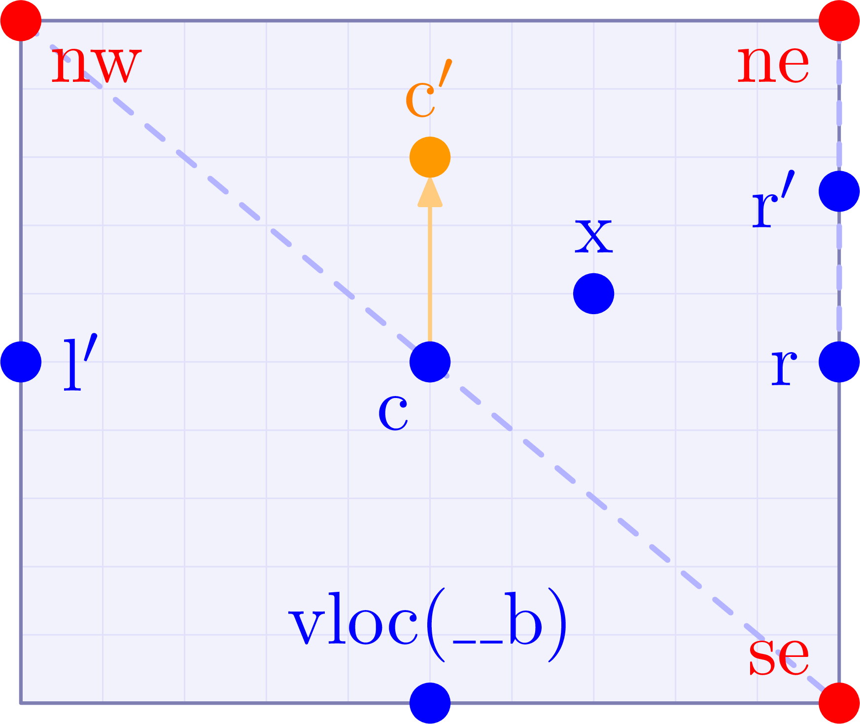
The usual “feynMF vertices” declared with \fmfleft, \fmfright, etc. are stored in a special dictionary. Their corresponding MetaPost pair can be accessed in MetaPost by prepending its label with two underscores and using the lookup function called vloc. Below are some examples.
\documentclass[11pt,border=4pt]{standalone}
\usepackage{feynmp-auto}
\begin{document}
\begin{fmffile}{feyngraph}
  \begin{fmfgraph*}(120,100) % dimensions (WH)
    % predefined points (MetaPost pairs)
    \fmfiv{d.sh=circle,d.f=1,d.si=5pt,l.a=-45,l=nw}{nw}
    \fmfiv{d.sh=circle,d.f=1,d.si=5pt,l.a=-135,l=ne}{ne}
    \fmfiv{d.sh=circle,d.f=1,d.si=5pt,l.a=135,l=se}{se}
    % define (external) vertices
    \fmfleft{l}
    \fmfright{r}
    \fmfbottom{b}
    % define vertices at exact point
    \fmfforce{(0.7w,0.6h)}{x} % at exact coordinates
    \fmfforce{0.5[nw,se]}{c}  % at midway between nw and se
    \fmfforce{c+(0,0.3h)}{c'} % at midway between nw and se
    \fmfforce{0.5[vloc(__r),ne]}{r'} % at midway between nw and r
    % convert feynmp vertex to MetaPost pair
    \fmfipair{l'} % declare MetaPost pair
    \fmfiequ{l'}{vloc(__l)} % convert
    % draw new points with labels
    \fmfiv{d.sh=circle,d.f=1,d.si=5pt,l.a=0,l=l$'$}{l'}
    \fmfiv{d.sh=circle,d.f=1,d.si=5pt,l.a=90,l={vloc(\_\_b)}}{vloc(__b)}
    \fmfv{d.sh=circle,d.f=1,d.si=5pt,l.a=-170,l=r}{r}
    \fmfv{d.sh=circle,d.f=1,d.si=5pt,l.a=-170,l=r$'$}{r'}
    \fmfv{d.sh=circle,d.f=1,d.si=5pt,l.a=90,l=x}{x}
    \fmfv{d.sh=circle,d.f=1,d.si=5pt,l.a=-120,l=c}{c}
    \fmfv{d.sh=circle,d.f=1,d.si=5pt,l.a=90,l=c$'$}{c'}
  \end{fmfgraph*}
\end{fmffile}
\end{document}
You can find an example in the previous tutorial on placing vertices with \fmfforce.
Lines: MetaPost paths
Straight lines & path manipulations
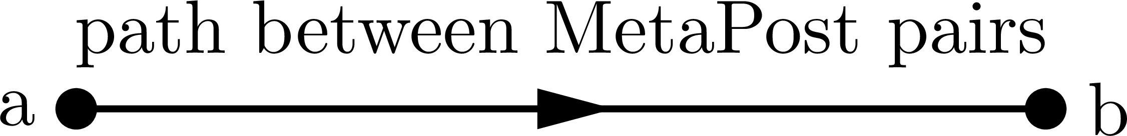
Here is the simplest way to draw a straight line between two points using the intermediate \fmfi:
\documentclass[11pt,border=15pt]{standalone}
\usepackage{feynmp-auto}
\begin{document}
\begin{fmffile}{feyngraph}
  \begin{fmfgraph*}(140,20) % dimensions (WH)
    % declare MetaPost pairs
    \fmfipair{a,b}
    % set MetaPost pairs
    \fmfiequ{a}{(0,0)}
    \fmfiequ{b}{(1w,0)}
    % label MetaPost pairs
    \fmfiv{d.sh=circle,d.f=1,d.si=5pt,l=a,l.a=180}{a}
    \fmfiv{d.sh=circle,d.f=1,d.si=5pt,l=b,l.a=0}{b}
    % draw line
    \fmfi{fermion,l=path between MetaPost pairs,l.s=left}{a--b}
  \end{fmfgraph*}
\end{fmffile}
\end{document}
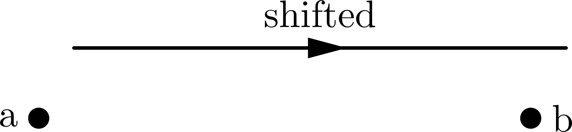
It is important to realize that the last argument to \fmfi is basically a draw command in MetaPost. One can therefore define do other manipulations like shift or rotate:
\documentclass[11pt,border=15pt]{standalone}
\usepackage{feynmp-auto}
\begin{document}
\begin{fmffile}{feyngraph}
  \begin{fmfgraph*}(140,38) % dimensions (WH)
    % declare MetaPost pairs
    \fmfipair{a,b}
    % set MetaPost pairs
    \fmfiequ{a}{(0,0)}
    \fmfiequ{b}{(1w,0)}
    % label MetaPost pairs
    \fmfiv{d.sh=circle,d.f=1,d.si=5pt,l=a,l.a=180}{a}
    \fmfiv{d.sh=circle,d.f=1,d.si=5pt,l=b,l.a=0}{b}
    % draw line
    \fmfi{fermion,l=shifted,l.s=left}{(a--b) shifted(10,20)}
  \end{fmfgraph*}
\end{fmffile}
\end{document}
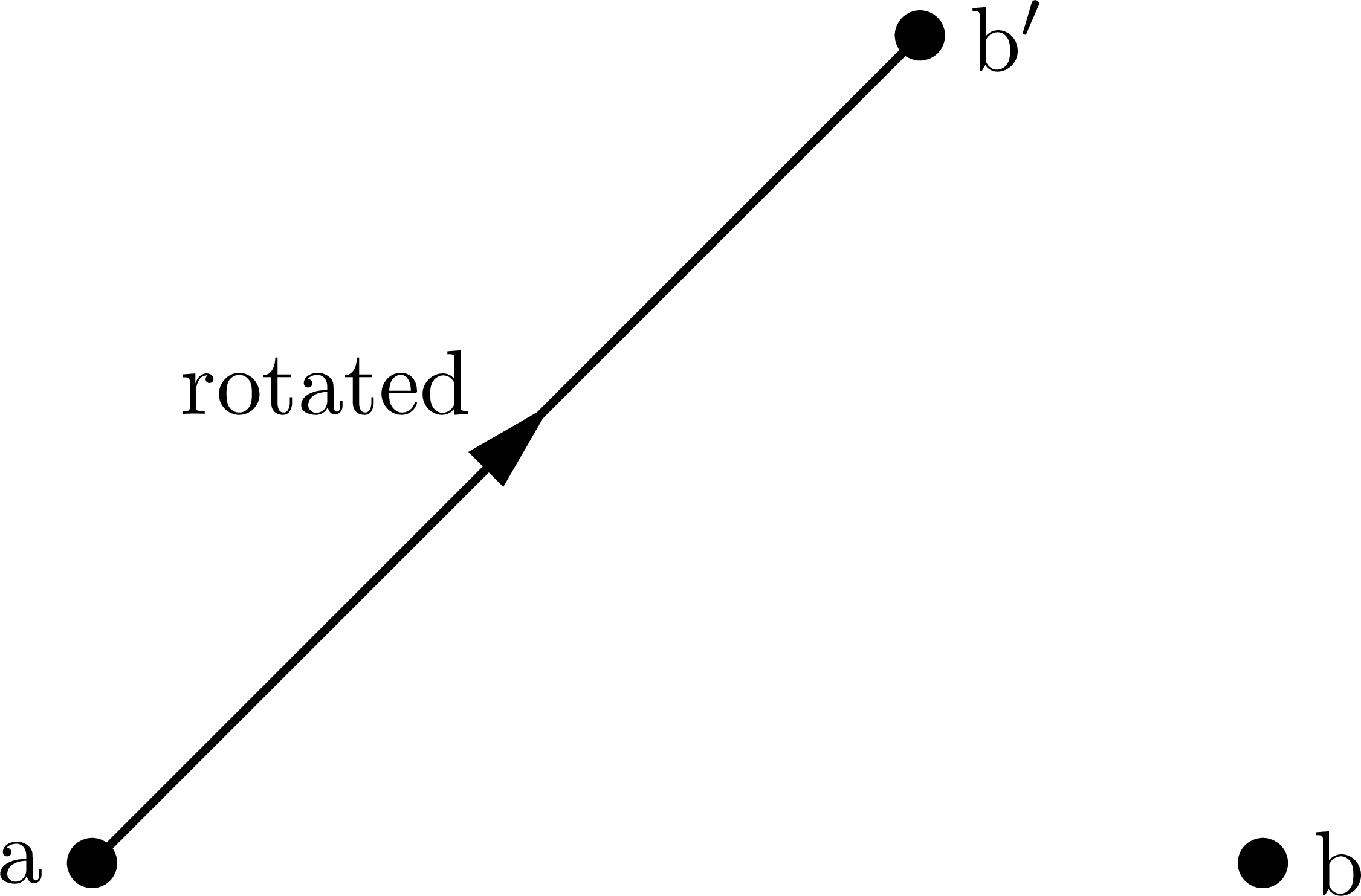
An example of rotating a line around some point:
\documentclass[11pt,border=15pt]{standalone}
\usepackage{feynmp-auto}
\begin{document}
\begin{fmffile}{feyngraph}
  \begin{fmfgraph*}(140,110) % dimensions (WH)
    % declare MetaPost pairs
    \fmfipair{a,b,b'}
    % set MetaPost pairs
    \fmfiequ{a}{(0,0)}
    \fmfiequ{b}{(1w,0)}
    \fmfiequ{b'}{b rotatedaround(a,45)}
    % label MetaPost pairs
    \fmfiv{d.sh=circle,d.f=1,d.si=5pt,l=a,l.a=180}{a}
    \fmfiv{d.sh=circle,d.f=1,d.si=5pt,l=b,l.a=0}{b}
    \fmfiv{d.sh=circle,d.f=1,d.si=5pt,l=b$'$,l.a=0}{b'}
    % draw line
    \fmfi{fermion,l=rotated,l.s=left}{(a--b) rotatedaround(a,45)}
  \end{fmfgraph*}
\end{fmffile}
\end{document}
Curved lines
There are several common methods of making curved paths in intermediate mode.
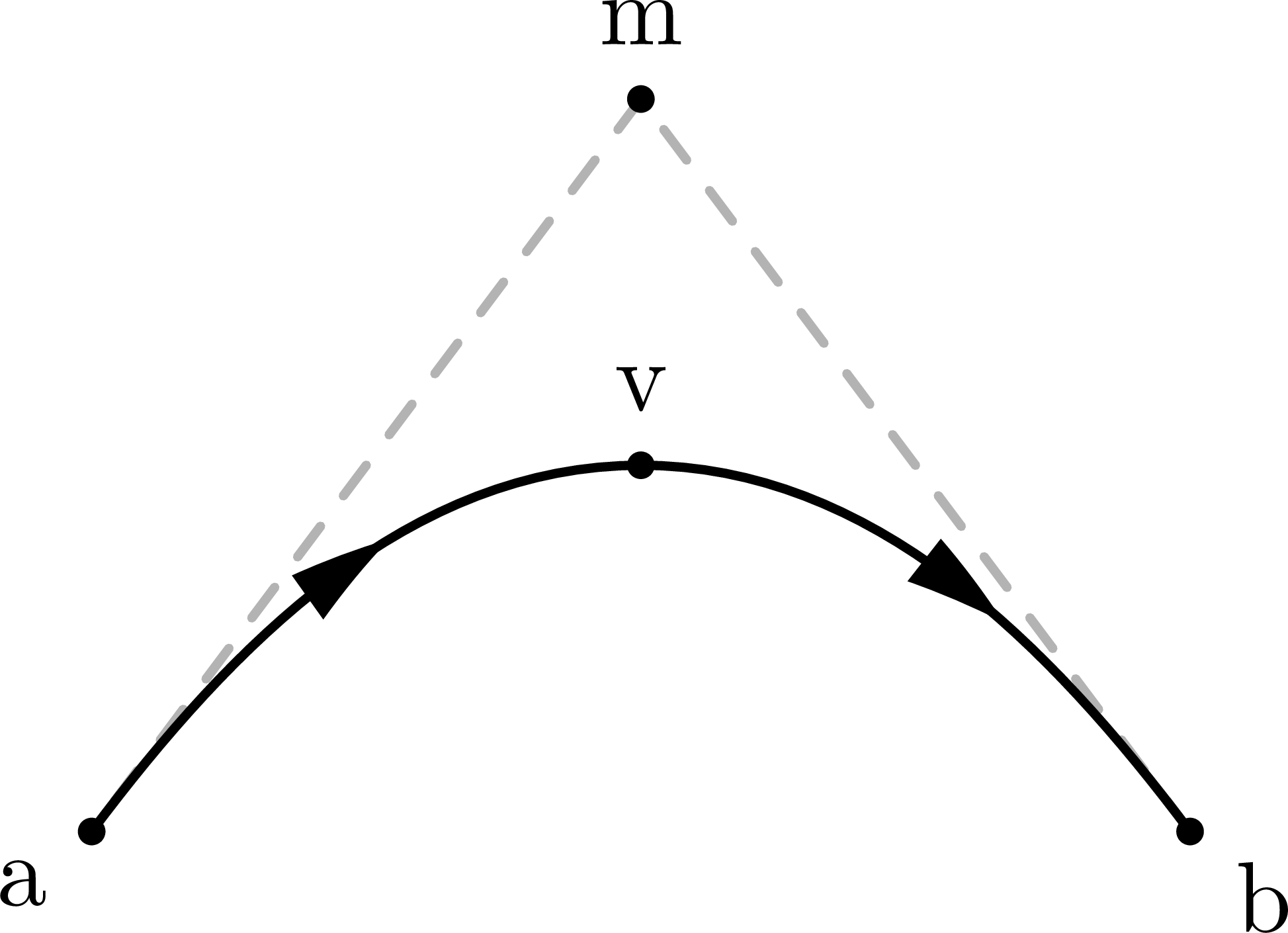
Below is an example of drawing curved paths with MetaPost syntax:
    \fmfi{fermion}{a{m-a} .. {right}v}

    \fmfi{fermion}{v{right} .. {b-m}b}
The first line draws a path from a to v. The .. operator connects these points with a smoothly curved path. With curly braces before or after a point, one can define at which angle the curved line starts or ends, respectively:
-
a{m-a}means that the linem-ais the tangent of the path starting in pointatowardsm. -
{right}vmeans the curved path ends in pointv, while going in the right/east direction. An equivalent method would be to write{dir 0}v, because the line arrives with a tangent that makes an angle of 0° with respect to the horizontal.
\documentclass[11pt,border=15pt]{standalone}
\usepackage{feynmp-auto}
\begin{document}
\begin{fmffile}{feyngraph}
  \begin{fmfgraph*}(120,80) % dimensions (WH)
    % declare MetaPost pairs
    \fmfipair{a,b,v,m}
    % set MetaPost pairs
    \fmfiequ{a}{(0,0)}
    \fmfiequ{b}{(w,0)}
    \fmfiequ{v}{(.5w,.5h)}
    \fmfiequ{m}{(.5w,h)}
    % draw grey tangent line (for illustration purposes)
    \fmfi{dashes,foreground=(0.7,,0.7,,0.7)}{m--a}
    \fmfi{dashes,foreground=(0.7,,0.7,,0.7)}{b--m}
    % draw curved paths
    \fmfi{fermion}{a{m-a} .. {right}v}
    \fmfi{fermion}{v{right} .. {b-m}b}
    %\fmfi{fermion}{a{m-a} .. {dir 0}v} % equivalent
    % label points
    \fmfiv{d.sh=circle,d.f=1,d.si=2pt,l=a}{a}
    \fmfiv{d.sh=circle,d.f=1,d.si=2pt,l=b}{b}
    \fmfiv{d.sh=circle,d.f=1,d.si=2pt,l=m}{m}
    \fmfiv{d.sh=circle,d.f=1,d.si=2pt,l=v,l.a=90}{v}
  \end{fmfgraph*}
\end{fmffile}
\end{document}
\documentclass[11pt,border=15pt]{standalone}
\usepackage{feynmp-auto}
\begin{document}
\begin{fmffile}{feyngraph}
\begin{fmfgraph*}(80,80) % dimensions (WH)
% draw curved path
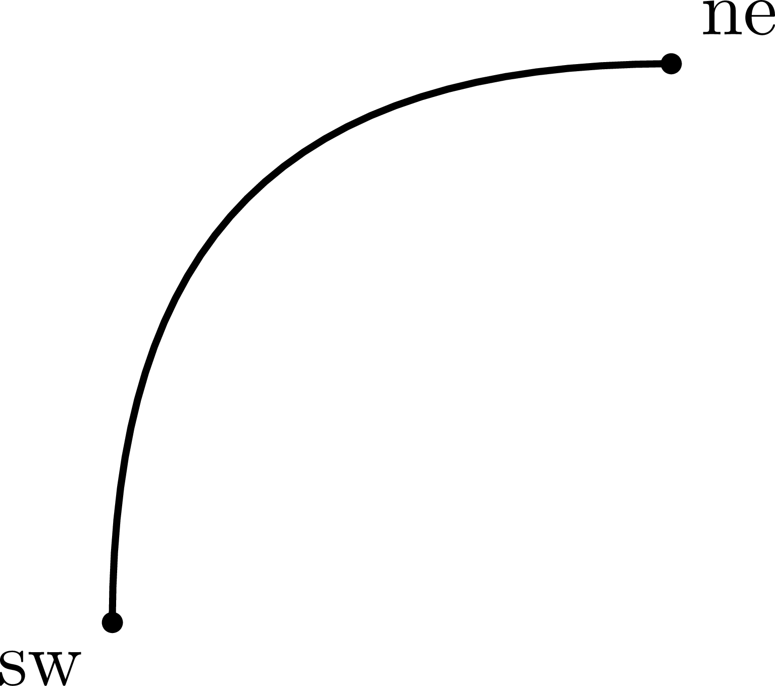
\fmfi{plain}{sw{up} .. tension .8 .. {right}ne}
% label points
\fmfiv{d.sh=circle,d.f=1,d.si=2pt,l=sw}{sw}
\fmfiv{d.sh=circle,d.f=1,d.si=2pt,l=ne}{ne}
\end{fmfgraph*}
\end{fmffile}
\end{document}
\documentclass[11pt,border=15pt]{standalone}
\usepackage{feynmp-auto}
\begin{document}
\begin{fmffile}{feyngraph}
\begin{fmfgraph*}(80,80) % dimensions (WH)
% draw curved path
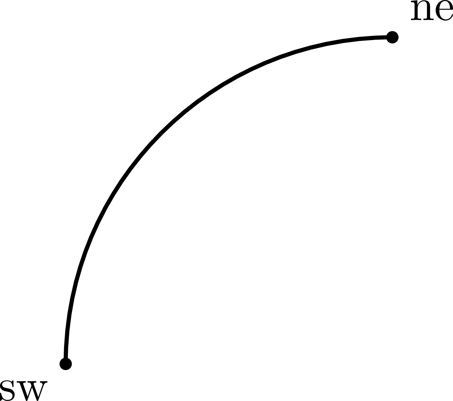
\fmfi{plain}{sw{up} .. {right}ne}
%\fmfi{plain}{sw{up} .. tension 1 .. {right}ne} % equivalent
% label points
\fmfiv{d.sh=circle,d.f=1,d.si=2pt,l=sw}{sw}
\fmfiv{d.sh=circle,d.f=1,d.si=2pt,l=ne}{ne}
\end{fmfgraph*}
\end{fmffile}
\end{document}
\documentclass[11pt,border=15pt]{standalone}
\usepackage{feynmp-auto}
\begin{document}
\begin{fmffile}{feyngraph}
\begin{fmfgraph*}(80,80) % dimensions (WH)
% draw curved path
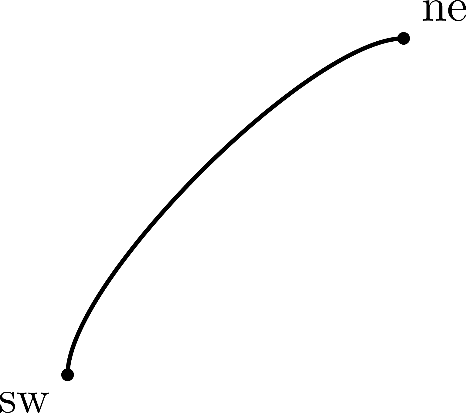
\fmfi{plain}{sw{up} .. tension 2 .. {right}ne}
% label points
\fmfiv{d.sh=circle,d.f=1,d.si=2pt,l=sw}{sw}
\fmfiv{d.sh=circle,d.f=1,d.si=2pt,l=ne}{ne}
\end{fmfgraph*}
\end{fmffile}
\end{document}
\documentclass[11pt,border=15pt]{standalone}
\usepackage{feynmp-auto}
\begin{document}
\begin{fmffile}{feyngraph}
\begin{fmfgraph*}(160,80) % dimensions (WH)
% curved path
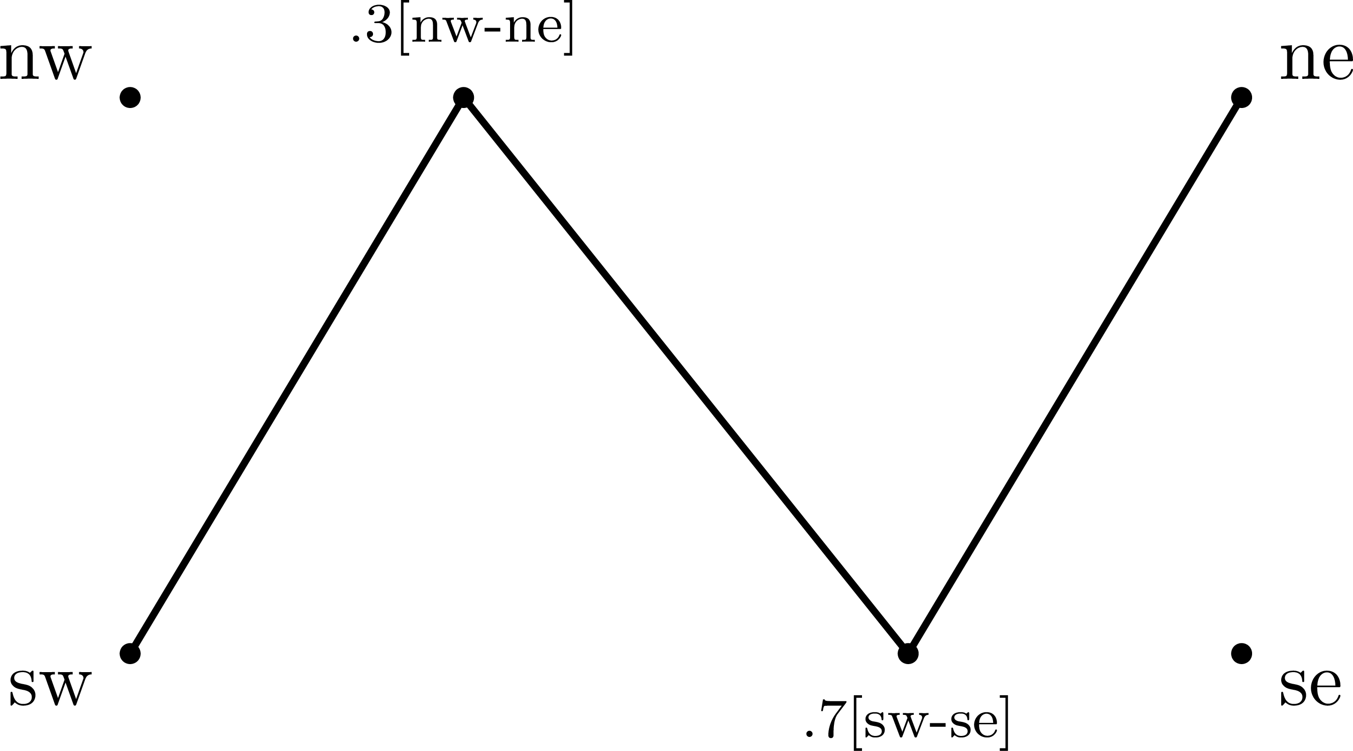
\fmfi{plain}{sw -- .3[nw,ne] -- .7[sw,se] -- ne}
% point labels
\fmfiv{d.sh=circle,d.f=1,d.si=2pt,l=nw}{nw}
\fmfiv{d.sh=circle,d.f=1,d.si=2pt,l=ne}{ne}
\fmfiv{d.sh=circle,d.f=1,d.si=2pt,l=sw}{sw}
\fmfiv{d.sh=circle,d.f=1,d.si=2pt,l=se}{se}
\fmfiv{d.sh=circle,d.f=1,d.si=2pt,l=\scriptsize.3[nw-ne],l.a=90}{.3[nw,ne]}
\fmfiv{d.sh=circle,d.f=1,d.si=2pt,l=\scriptsize.7[sw-se],l.a=-90}{.7[sw,se]}
\end{fmfgraph*}
\end{fmffile}
\end{document}
\documentclass[11pt,border=15pt]{standalone}
\usepackage{feynmp-auto}
\begin{document}
\begin{fmffile}{feyngraph}
\begin{fmfgraph*}(160,80) % dimensions (WH)
% curved path
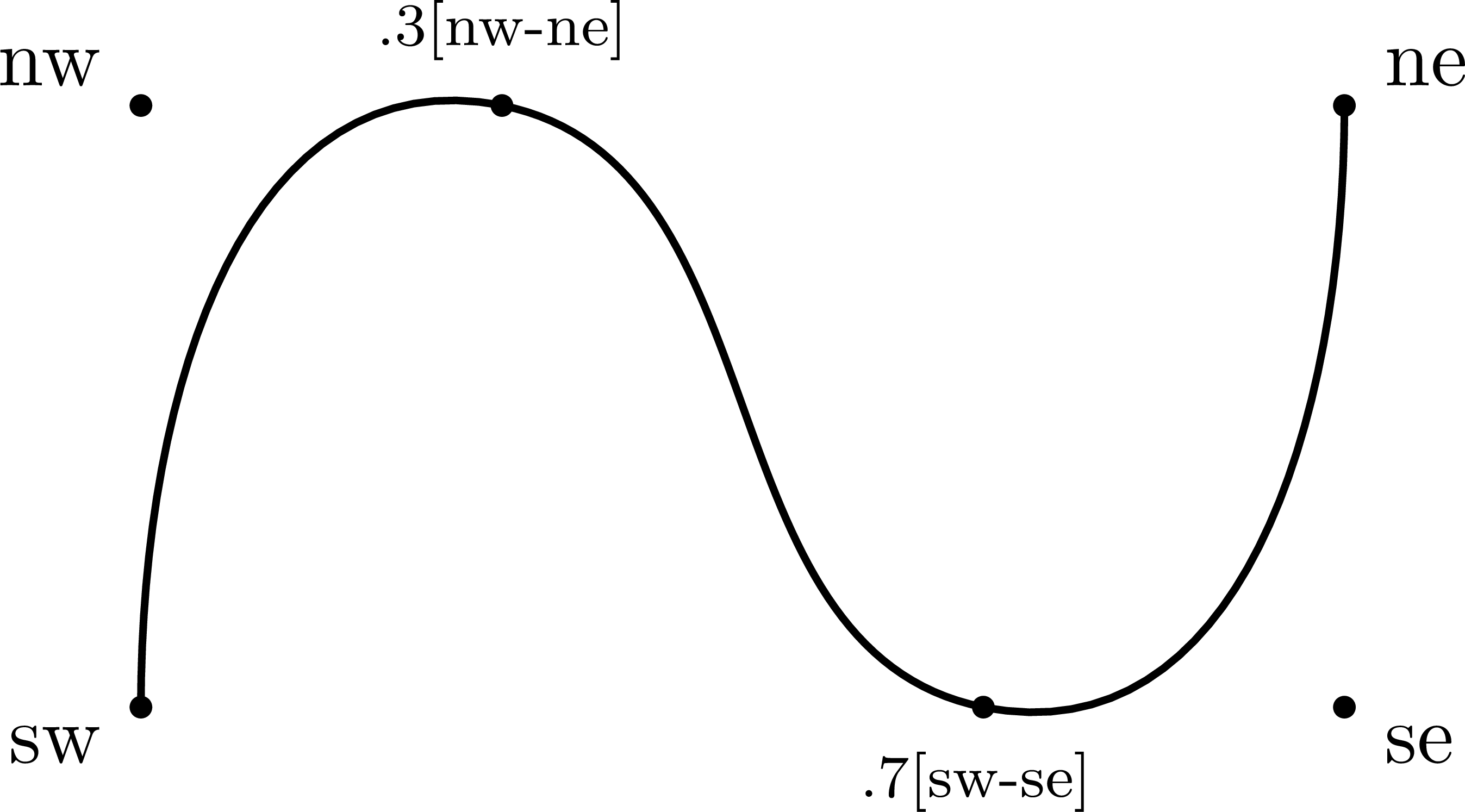
\fmfi{plain}{sw{up} .. .3[nw,ne] .. .7[sw,se] .. {up}ne}
% point labels
\fmfiv{d.sh=circle,d.f=1,d.si=2pt,l=nw}{nw}
\fmfiv{d.sh=circle,d.f=1,d.si=2pt,l=ne}{ne}
\fmfiv{d.sh=circle,d.f=1,d.si=2pt,l=sw}{sw}
\fmfiv{d.sh=circle,d.f=1,d.si=2pt,l=se}{se}
\fmfiv{d.sh=circle,d.f=1,d.si=2pt,l=\scriptsize.3[nw-ne],l.a=90}{.3[nw,ne]}
\fmfiv{d.sh=circle,d.f=1,d.si=2pt,l=\scriptsize.7[sw-se],l.a=-100}{.7[sw,se]}
\end{fmfgraph*}
\end{fmffile}
\end{document}
\documentclass[11pt,border=15pt]{standalone}
\usepackage{feynmp-auto}
\begin{document}
\begin{fmffile}{feyngraph}
\begin{fmfgraph*}(160,80) % dimensions (WH)
% curved path
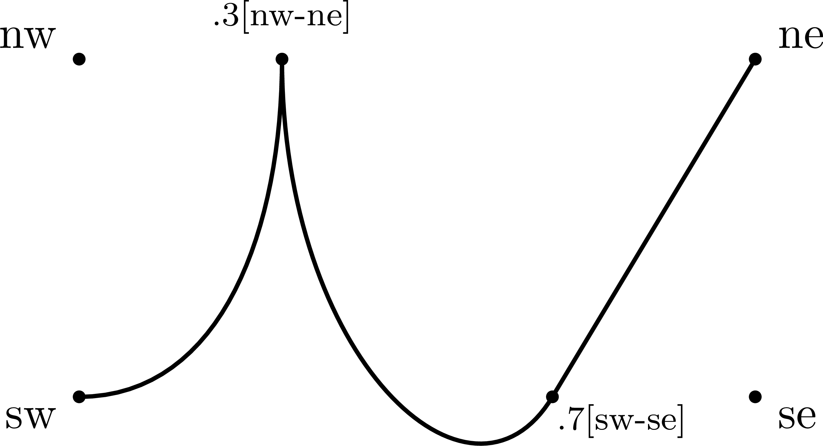
\fmfi{plain}{sw{right} .. {up}.3[nw,ne]{down} .. .7[sw,se] --- ne}
% point labels
\fmfiv{d.sh=circle,d.f=1,d.si=2pt,l=nw}{nw}
\fmfiv{d.sh=circle,d.f=1,d.si=2pt,l=ne}{ne}
\fmfiv{d.sh=circle,d.f=1,d.si=2pt,l=sw}{sw}
\fmfiv{d.sh=circle,d.f=1,d.si=2pt,l=se}{se}
\fmfiv{d.sh=circle,d.f=1,d.si=2pt,l=\scriptsize.3[nw-ne],l.a=90}{.3[nw,ne]}
\fmfiv{d.sh=circle,d.f=1,d.si=2pt,l=\scriptsize.7[sw-se],l.a=-60,l.d=2}{.7[sw,se]}
\end{fmfgraph*}
\end{fmffile}
\end{document}

")


 in pp")